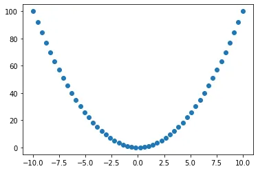
A Dense layer

A dense layer is essentially a set of weights and biases applied to the input wrapped in an activation function

In the y = x² example we have a single input x and we would apply a weight w and bias b then wrap that in an activation function a giving us..

a(wx + b)

depending on how many units / nodes we want our dense layer to have we can just repeat this with different weights & biases giving us

[a(w₀x + b₀),
 a(w₁x + b₁), 
 ... 
 a(wₙx + bₙ)]

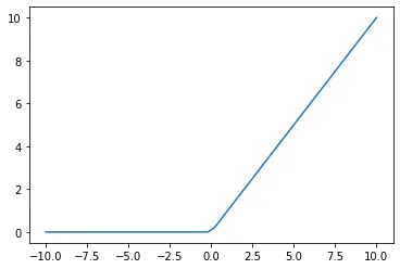
The Activation Function: There are a few different ones, but we are going to focus on relu which is really simple.

relu(x) = x if x > 0 else 0

Learning y = x²

You might be wondering… how this dense layer is ever going to figure out a non-linear relationship like x² given it’s seemingly linear operations.

So.. suppose you have a Dense(2) layer (dense layer with two nodes), and keep the weights as 1 and biases as 0 for simplicity

Dense(2) layernode 0 = a(w₀x + b₀) = relu(x)node 1 = a(w₁x + b₁) = relu(-x)

if we fed those outputs into a Dense(1) layer with a linear activation function (a(x) = x) we would get (and again keeping the weights and biases to 1 and 0)

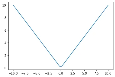
Dense(1) layer (linear activation function a(x) = x)node 0 = a(w₀relu(x) + b₀) + a(w₁relu(-x) + b₁) 
node 0 = relu(x) + relu(-x)

plotting this is starting to look promising..

So our machine learning topology would be a Dense(2) layer with relu activation function, connected to a Dense(1) layer with a linear activation function.

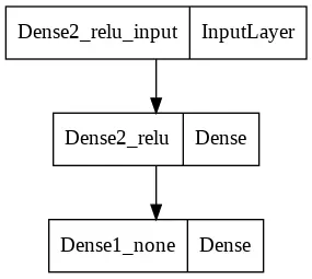
Here is how you would define that in Tensorflow

model = keras.Sequential([
  layers.Dense(units = 2, activation = 'relu'),
  layers.Dense(1, activation = None)
])

Hopefully you can start to see how this whole ML stuff might work… you decompose complicated relationships into a series of linear functions, stacked on top of each other with a non-linear activation function like relu.

Increasing the nodes

So as you might have guessed we can get a better model by increasing the number of nodes / units in our first Dense layer

Here is an example in Tensorflow, trained using Mean Squared Error loss

import tensorflow as tf
from tensorflow import keras
from tensorflow.keras import layersimport numpy as np 
import matplotlib
from matplotlib import pyplot as pltm1 = keras.Sequential([
  # need this to flatten the input [1,2,3] => [[1],[2],[3]]
  layers.Flatten(), 
  layers.Dense(units = 4, 
               activation = 'relu'), 
  layers.Dense(1)
])m1.compile(
    loss=tf.keras.losses.MSE,
    optimizer=tf.optimizers.Adam(learning_rate=0.01))m1.fit(x, y, epochs=1000, batch_size=10, verbose=0)# plot the results 
plt.plot(x , y)
plt.plot(x, m1(x))

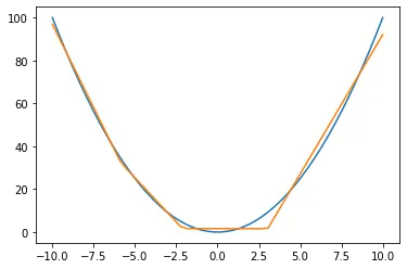
Lets look under the hood at the 4 lines generated by the first dense layer

# Get our 1st dense layer 
l = m1.layers[1] 
# get x in the shape expected by the layer 
x1 = x.reshape((-1, 1)) 
# apply the layer weights and bias 
y1 = (np.dot(x1, l.kernel.numpy()) + l.bias.numpy())
# apply relu 
y1[y1 < 0] = 0 
# plot lines 
plt.plot(x, y1)

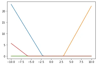
You can really see, how adding these together can start approximating y = x²

The machine learning bit

So now you understand how dense layers can be stacked to generate non-linear patterns, I’ll touch on how we figure out our weights and biases for these lines.

The basic idea is very similar to regression, in fact we are using the same loss function in this model. Mean Squared Error.

So the loss function here is defined by

loss = (y₀ - m(x₀))² + (y₁ - m(x₁))² + ... + (yₙ - m(xₙ))²where m is our modelm(x) = w₀m₀(x) + b₀ + .. + w₀m₃(x) + b₃and mᵢ is our 1st dense layer mᵢ(x) = wᵢx + bᵢ

Which essentially gives us some polynomial equation dependent on the 4 weights and biases of our first dense layer, and the 4 weights and biases of our second layer

without going into too much detail we can easily estimate the gradient at a particular point in our 8 dimensional space and start moving in the direction of the minimal point.

Obviously there is no guarantee that our 8 dimensional space as only 1 minimal point, there maybe local minima that we get stuck in.

So machine learning models, try to tread carefully by not moving too quickly to the identified minimal point (specified somewhat by the learning_rate, selection of the batch size and epochs)