Project 2 - Rankine cycle Simulator

Objective:
1) Creating a Rankine Cycle Simulator & Calculating the state points of the Rankine
Cycle based on user inputs.
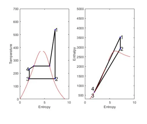
2) Plotting the corresponding T-S and H-S plots for the given set of inputs
Rankine Cycle:
The Rankine cycle is a model used to predict the performance of steam turbine
systems. It was also used to study the performance of reciprocating steam engines.
The Rankine cycle is an idealized thermodynamic cycle of a heat engine that
converts heat into mechanical work while undergoing phase change. It is an idealized
cycle in which friction losses in each of the four components are neglected. The heat
is supplied externally to a closed loop, which usually uses water as the working fluid
Processes in Rankine Cycle:
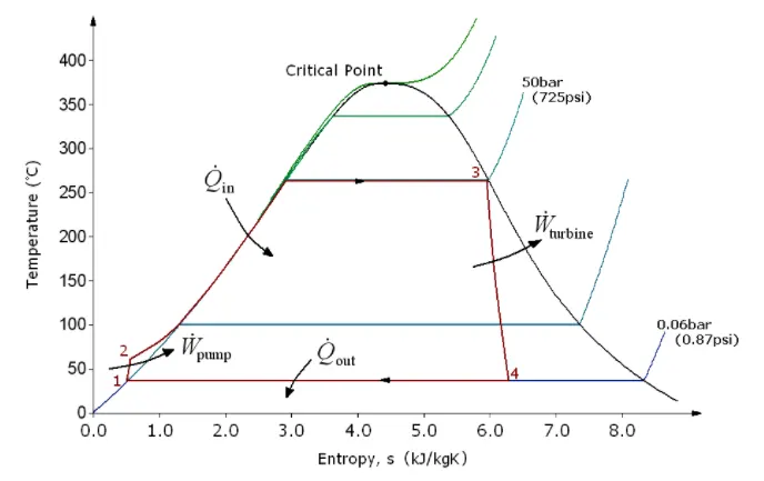
There are four processes in the Rankine cycle. These states are identified by numbers
(in brown) in the above T–s diagram.
Process 1–2: The working fluid is pumped from low to high pressure. As the
fluid is a liquid at this stage, the pump requires little input energy.
Process 2–3: The high-pressure liquid enters a boiler, where it is heated at
constant pressure by an external heat source to become a dry saturated
vapour. The input energy required can be easily calculated graphically, using
an enthalphy-entropy chart , or Mollier Diagram), or numerically, using steam
tables
Process 3–4: The dry saturated vapour expands through a turbine, generating
power. This decreases the temperature and pressure of the vapour, and some
condensation may occur. The output in this process can be easily calculated
using the chart or tables noted above.
Process 4–1: The wet vapour then enters a condenser, where it is condensed
at a constant pressure to become a saturated liquid

Procedure
1.We will use standard Xsteam library to get the steam table data for water, is given
below. It must be used to calculate the points in between the state variables.
2. Clearing workspace, command window & closing all plots
3. The user inputs that have to be entered by the user are:
Pressure at the turbine inlet (in bar)
Temperature at the turbine inlet (in Degree C)
Pressure at the Condenser(in bar)
4. Based on the inputs we will calculate state variables by using equation of state and
X_steam library which is a steam table and we can directly read values of state
variables using it.
5.After calculating the state variables at each state point we have calculated the
turbine and pump work done.
6. At the end we plotted the corresponding T-s and h-s plots for the given set of
inputs.
Matlab Code:
close all
clear all
clc
%Simulating Rankine Cycle
% Process Description
fprintf('1‐2 Isobaric heat Transfer\n')
fprintf('2‐3 Isentropic Expansion\n')
fprintf('2‐3 Isentropic Expansion\n')
fprintf('3‐4 Isobaric heat Rejection\n')
fprintf('4‐1 Isentropic Compression\n')
%Inputs
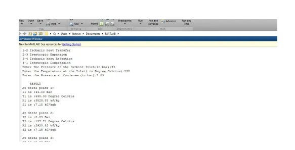
p1 = input('Enter the Pressure at the turbine Inlet(in bar):');
t1 = input( 'Enter the Temperature at the Inlet( in Degree Celcius):');
p2 = input('Enter the Pressure at Condenser(in bar):');
%Input Conditions
t = XSteam('Tsat_p',p1);
if t1>=t
h1 = XSteam('h_pT',p1,t1);
s1 = XSteam('s_pT',p1,t1);
%State points Evaluation
p4 = p1;
p3 = p2;
h3 = XSteam('hL_p',p3);
s3 = XSteam('sL_p',p3);
t3 = XSteam('Tsat_p',p3);
s2 = s1;
t2 = t3;
sf2 = XSteam('sL_p',p2);
sg2 = XSteam('sV_p',p2);
x2 = (s2 ‐ sf2)/(sg2 ‐ sf2);
hf2 = XSteam('hL_p',p2);
hg2 = XSteam('hV_p',p2);
h2 = hf2 + x2*(hg2 ‐ hf2);
s4 = s3;
h4 =XSteam('h_ps',p4,s4);
cp4 = XSteam('Cp_ps',p4,s4);
cv4 = XSteam('Cv_ps',p4,s4);
g4 = cp4/cv4;
o = (g4 ‐ 1)/g4;
t4 = t3*((p4/p3)^o);
%Turbine & Pump Work
wt = h1 ‐ h2;
wp = h4 ‐ h3;
%net work
wnet = wt ‐ wp;
%heat suppied
qs = h1 ‐ h4;
%Efficiency
n_per = (wnet/qs)*100;
n_per = (wnet/qs)*100;
%Steam rate per second
stm_rate = 3600/(wt ‐ wp);
%For process 4‐1, which is isobaric we use the expression dH=Cp*dT
t5 = XSteam('Tsat_p',p1);
s5 = XSteam('sL_p',p1);
s6 = XSteam('sV_p',p1);
%output
fprintf('\n\tRESULT\n')
fprintf('At State point 1:\nP1 is :%4.2f Bar\nT1 is :%4.2f Degree Celcius\nH1 is :%4.2f kJ/kg\nS1 is :%4.2f kJ/kgk\n\n',p1,t1,h1,s1)
fprintf('At State point 2:\nP2 is :%4.2f Bar\nT2 is :%4.2f Degree Celcius\nH2 is :%4.2f kJ/kg\nS2 is :%4.2f kJ/kgk\n\n',p2,t2,h2,s2)
fprintf('At State point 3:\nP3 is :%4.2f Bar\nT3 is :%4.2f Degree Celcius\nH3 is :%4.2f kJ/kg\nS3 is :%4.2f kJ/kgk\n\n',p3,t3,h3,s3)
fprintf('At State point 4:\nP4 is :%4.2f Bar\nT4 is :%4.2f Degree Celcius\nH4 is :%4.2f kJ/kg\nS4 is :%4.2f kJ/kgk\n\n',p4,t4,h4,s4)
fprintf('Wt is :%4.2f kJ/kg\nWp is :%4.2f kJ/kg\nWnet is :%4.2f kJ/kg\nNtherm is :%4.2f percent\nS.S.C is :%4.2f kg/kWh',wt,wp,wnet,n_per,stm_rate)
%Vapour line
temp = linspace(1,400,100);
for i=1:length(temp)
ent_l(i) = XSteam('sL_T',temp(i));
ent_v(i) = XSteam('sV_T',temp(i));
enth_l(i) = XSteam('hL_T',temp(i));
enth_v(i) = XSteam('hV_T',temp(i));
end
%Plotting
subplot(1,2,1)
plot([s1 s2 s3 s4 s5 s6 s1],[t1 t2 t3 t4 t5 t5 t1],'color','k','linewidth',2,'marker','o','markersize',2,'markerfacecolor','b','markeredgecolor','b')
hold on
plot(ent_l,temp,'color','r')
plot(ent_v,temp,'color','r')
axis([0 10 0 700])
text(s1,t1,'1','FontSize',15)
text(s2,t2,'2','FontSize',15)
text(s3,t3,'3','FontSize',15,'HorizontalAlignment','right')
text(s4,t4,'4','FontSize',15,'HorizontalAlignment','right')
xlabel('Entropy')
ylabel('Temperature')
subplot(1,2,2)
plot([s1 s2 s3 s4 s1],[h1 h2 h3 h4 h1],'color','k','linewidth',2,'marker','o','markersize',2,'markerfacecolor','b','markeredgecolor','b')
axis([0 10 300 5000])
hold on
plot(ent_v,enth_v,'color','r')
plot(ent_l,enth_l,'color','r')
text(s1,h1,'1','FontSize',15)
text(s2,h2,'2','FontSize',15)
text(s2,h2,'2','FontSize',15)
text(s3,h3,'3','FontSize',15,'HorizontalAlignment','right','VerticalAlignment','top')
text(s4,h4,'4','FontSize',15,'HorizontalAlignment','right','VerticalAlignment','bottom')
xlabel('Entropy')
ylabel('Enthalpy')
else
fprintf('Enter Temperature Greater or Equal to Saturation Temperature')
end