Calculating the deformation of a two stepped bar using MatLab
AIM - Calculating the deformation of the stepped Bar by FEA Approach in Matlab
OBJECTIVES :
To write a MATLAB Program, calculating the deformation of the Stepped Bar deformation due to applied axial force by the FEM method.
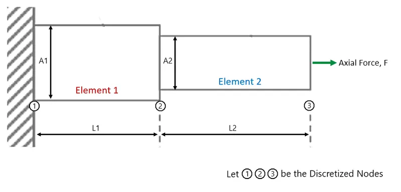
Take, Stepped bar of 2 elements of square cross-sections with one end is clamped or fixed support and other end applied an axial force, as the example shown below -
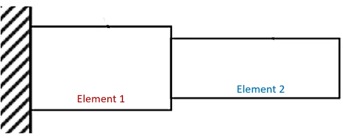
Scope the project -
- The stepped bar solver will be for only two elements stepped bar.
- This program is applicable only for square Cross-section stepped bar.
- Deformation is only in one direction i.e. axially is considered.
- Basic Simulation of the deformation
THEORY :
Strength of Materials –
The strength of a material is its ability to withstand an applied load without failure or plastic deformation. The field of strength of materials deals with forces and deformations that result from their acting on a material.
Deformation -
is a change of the dimensions and in some case shape of a body due to an applied external force.
Young's Modulus or Modulus of Elasticity -
Young modulus, or the modulus of elasticity in tension, is a mechanical property that measures the tensile stiffness of a solid material. It quantifies the relationship between tensile stress (force per unit area) and axial strain (proportional deformation) in the linear elastic region of a material.
Young's Modulus , `E = (STRESS)/(STRAIN) = (FORCE *AREA)/(LENGTH*DEFORMATION)`
`E = sigma/epsilon = (F.A)/(L.delta)`
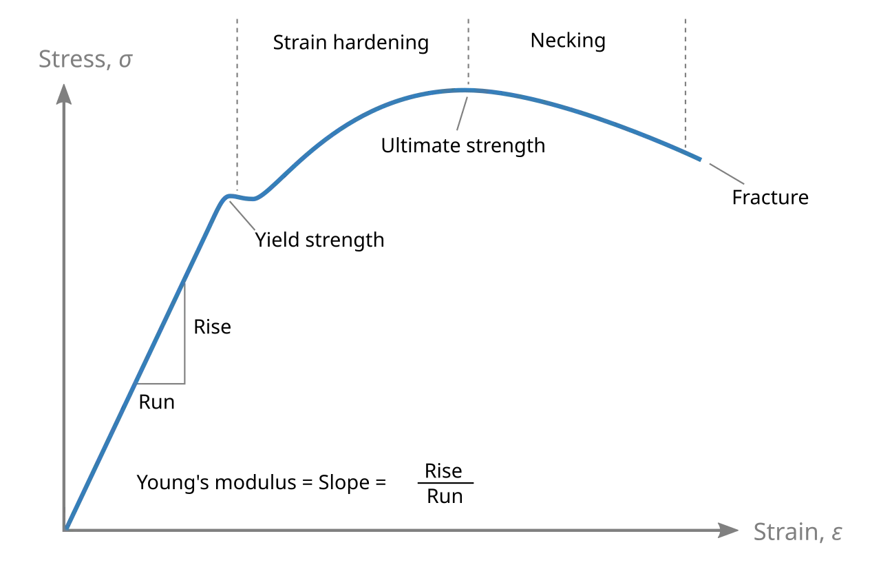
Deformation of Stepped Bar -
By Theoretical Method of Strength of Material (Solid Mechanics) -
The deformation of a structural member, with known geometry, and subjected to an axial load can be determined by using the following equation derived by the Young's Modulus -
`delta = (PL)/(EA)`
where, `delta` = Deformation or Displacement
P = Applied Axial Force (in Newtons)
L = Length of the structural member
E = Young's Modulus or Modulus of Elasticity
A = Cross-Section Area of the Structural member
The term EA/L is the stiffness of the member so we can rewrite the
equation as -
`delta = (P)/(k)`
where, `k = L/(EA)`
Therefore now in the Stepped Bar Problem,
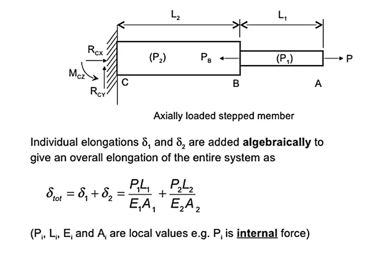
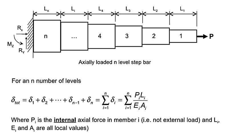
By Numerical or Computational Method of FEA -
Finite Element Analysis or FEA is the simulation of a physical phenomenon using a numerical mathematic technique referred to as the Finite Element Method, or FEM. This process is at the core of mechanical engineering, as well as a variety of other disciplines.
The finite element method is the representation of a body or a structure by an assemblage of sub-divisions called as finite elements. These elements are interconnected at joints which are called nodes or nodal points. Simple functions are chosen to approximate the distribution of actual displacements over each finite element. Such assumed functions are called displacement functions or displacement models. The unknown magnitude of the displacement functions are the displacements at the nodal points. Hence the final solutions will yield the approximate displacements at discrete locations in the body at the nodal points. A displacement model can be expressed in various forms, such as polynomials and trigonometric functions.
Steps -
1. Discretization into the element
Considering the same system or problem of Stepped Bar and discretizing into two Elements -
2. Selection of the displacement models
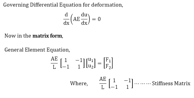
Here, we are considering just 1-D Deformation, and from the equation,
`delta or U= (FL)/(EA)`
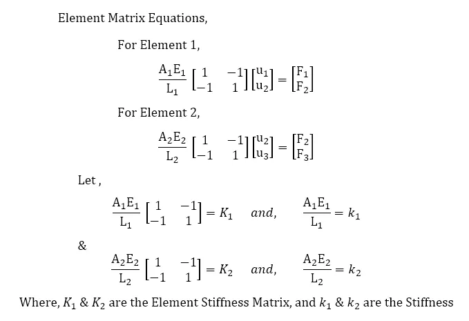
3. Derivation of the element stiffeness matrix.
4. Assembling
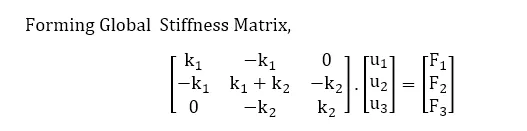
`K . U= F`
5. Solution for the unknown displacement
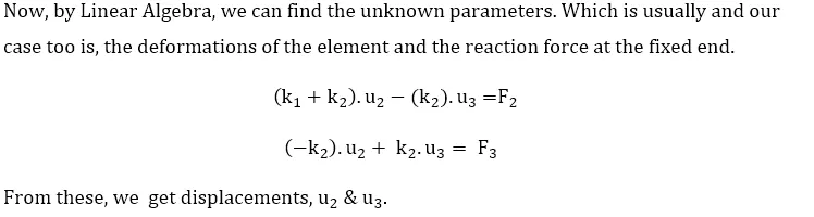
6. Computations of the element stresses or reaction forces at the nodal points
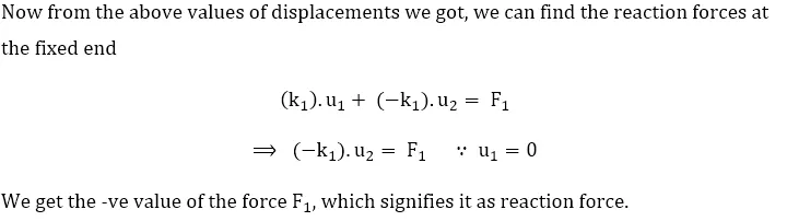
CONSIDERATION -
Considering the system and dimensions for our program, as shown below -
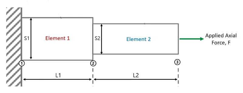
where, F = Applied Axial Force (in Newtons)
E = Young's Modulus or Modulus of Elasticity
S1 = Side length of the Element 1
S2 = Side length of the Element 2
A1 = Cross-Section Area of the Element 1 = S`1^2`
A2 = Cross-Section Area of the Element 2 = S`2^2`
L1 = Length of the 1st member or element
L2 = Length of the 2nd member or element
Let  be the Nodes, and F1, F2, F3, be the forces, u1, u2, u3 be the displacement, corresponding to nodes
clear all
close all
clc

fprintf('DEFORMATION CALCULATION OF 2 STEPPED BAR OF SQUARE C/S nn')

%========== dialogue box to enter the measurements of 1st stepped bar ==========

x = inputdlg({'Length in "mm" ','Width in "mm" ','Modulous of Elasticity in "N/mm^2" '},...
    'Details of 1st stepped bar',[1 50; 1 50; 1 50],{'100','50','200000'});

L1 = str2double(x{1}); W1 = str2double(x{2}); E1 = str2double(x{3});

fprintf('(1) Details of 1st stepped bar :-nn')
fprintf('  Length of 1st bar = %d mmn',L1)
fprintf('  Width of 1st bar = %d mmn',W1)
fprintf('  Modulous of elasticity = %d N/mm^2nn',E1)

%========== dialogue box to enter the measurements of 2nd stepped bar ==========

y = inputdlg({'Length in "mm" ','Width in "mm" ','Modulous of Elasticity in "N/mm^2" '},...
    'Details of 2nd stepped bar ',[1 50; 1 50; 1 50],{'100','30','200000'});

L2 = str2double(y{1}); W2 = str2double(y{2}); E2 = str2double(y{3});

fprintf('(2) Details of 2nd stepped bar :-nn')
fprintf('  Length of 2nd bar = %d mmn',L2)
fprintf('  Width of 2nd bar = %d mmn',W2)
fprintf('  Modulous of elasticity = %d N/mm^2nn',E2)

%================== Axial force acting on the two stepped bar ==================

f3 = inputdlg({'Axial Force in "Newtons" '},'Axial Force',[1 50],{'50000000'});

F = str2double(f3{1});
fprintf('(3) Force Applied(F) = %d Newtons nn',F)

%======================== Area of the two Stepped bars =========================

A1 = L1*W1;
fprintf(' Area of 1st bar(A1) = %d mm^2 n',A1)

A2 = L2*W2;
fprintf(' Area of 2nd bar(A2) = %d mm^2 n',A2)


I = [1 -1; -1 1]; % Identity Matrix

K1 = ((A1*E1)/L1)*I; % Stiffness matrix for element 1
K2 = ((A2*E2)/L2)*I;  % Stiffness matrix for element 2

% Global Stiffness matrix
K = [K1(1,1)    K1(1,2)    0;   K1(2,1)    K1(2,2)+K2(1,1)    K2(1,2);   0    K2(2,1)    K2(2,2)];

u1 = 0;   % At Node 1 the end of stepped bar is fixed therefore there can't be deflection
f2 = 0;   % Since we are considering the case in which the forcee is applied axialy on the other end only
          % therefore force at node 2 is considered 0

syms x y                            % assigns the symbols which can represented in the equations
eqn1 = K(2,2)*x + K(2,3)*y == 0;
eqn2 = K(3,2)*x + K(3,3)*y == f3;

sol = solve([eqn1,eqn2],[x,y]);    % Function solve() solves the to equation and give outputs of the variables

u2 = double(sol.x);
u3 = double(sol.y);

% calculating the Reaction force on the Node 1 using the obtained value of
% deforation and the global stiffness matrix
f1 = K(1,1)*u1 + K(1,2)*u2 + K(1,3)*u3;

fprintf(' n The Total Deformation / Displacement is = %f mm n',u3)
fprintf(' Deformation of 1st element is = %f mm n',u2)
fprintf(' Deformation of 2nd element is = %f mm n',u3-u2)
fprintf(' The Reaction force at the fixed end is = %d N n',f1)


% Simulatiing as Plot
p = (W1/2) - (W2/2);

x1 = u2/10;
x2 = u3/10;

Xaxis = L1+L2+200;
ct =1;
for j=1:4

    la1=L1;  la2=L2;    sa1=W1;  sa2=W2;

    for i=1:10
        L1 = L1 + x1;
        L2 = L2 + x2;
        hold on;
        plot([la1+la2 la1+la2],[-50 sa1+50],'--','linewidth',2,'color','g');
        title('Deformation of Square stepped bar due to Axial load');
        rectangle('position',[0,0,L1,W1],'facecolor',[0.800 0.1750 0.0980]);
        axis([0 Xaxis -50 W1+50]);
        rectangle('position',[L1,p,L2,W2],'facecolor',[0.05 0.450 0.750]);
        text(L1/4,W1/2,'Element 1');
        text(L1+L2/4,W1/2,'Element 2');

        grid on;
        pause(0.1);                 % by pause command it pauses the code there for provided time
        hold off;
        M(ct) = getframe(gcf);      % by getframe it Captures figure as movie frame
        ct = ct+1;
    end

    lb1=L1;  lb2=L2;    sb1=W1;  sb2=W2;
    for k=1:10

        L1 = L1 - x1;
        L2 = L2 - x2;
        hold on;
        plot([la1+la2 la1+la2],[-50 sa1+50],'--','linewidth',1,'color','g');
        plot([lb1+lb2 lb1+lb2],[-50 sb1+50],'--','linewidth',1,'color','r');
        legend('Deformation','Original Length');
        title('Deformation of Square stepped bar due to Axial load');
        rectangle('position',[0,0,L1,W1],'facecolor',[0.800 0.1750 0.0980]);
        axis([0 Xaxis -50 W1+50]);
        rectangle('position',[L1,p,L2,W2],'facecolor',[0.05 0.450 0.750]);
        text(L1/4,W1/2,'Element 1');
        text(L1+L2/4,W1/2,'Element 2');

        grid on;
        pause(0.1);                 % by pause command it pauses the code there for provided time
        hold off;
        M(ct) = getframe(gcf);      % by getframe it Captures figure as movie frame
        ct = ct+1;
        clf;
        plot([la1+la2 la1+la2],[-50 sa1+50],'--','linewidth',1,'color','g');
        plot([lb1+lb2 lb1+lb2],[-50 sb1+50],'--','linewidth',1,'color','r');
    end
    hold on;
end

movie(M);                % Play recorded movie frames
video = VideoWriter('SteppedBar_Deformation.avi','Uncompressed AVI'); % Write video files and assigning video file name and video format
video.FrameRate = 10;
open(video);            % Open file for writing video data
writeVideo(video,M);    % Write video data to file
close(video);           % Close file after writing video data
CODE EXPLANATION -
1)Taking required input from the user using input() commands -
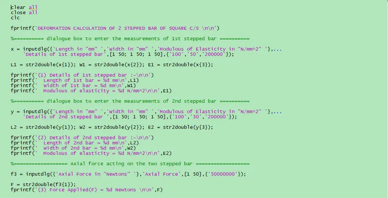
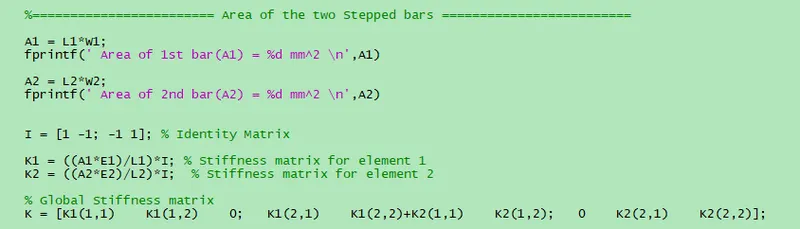
2) Here, the code is doing calculations based on the user input and known parameters and creating the Element and then Global stiffness matrices.
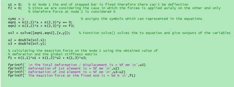
3)Now we using linear algebra we can find out the unknown variables, which are the deformations `u_2` and `'u_3`. And from the values of `u_2` & `'u_3`, we find the reaction force (F1) on the fixed end. Here in the following code, we used the tool syms and function solve() in order to form and solve the linear equation.
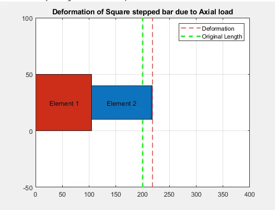
4)Following piece of code creates a movie of the simulation using the plot,-
Xaxis = L1+L2+200;
ct =1;
for j=1:4

    la1=L1;  la2=L2;    sa1=S1;  sa2=S2;

    for i=1:10
        L1 = L1 + x1;
        L2 = L2 + x2;
        hold on;
        plot([la1+la2 la1+la2],[-50 sa1+50],'--','linewidth',2,'color','g');
        title('Deformation of Square stepped bar due to Axial load');
        rectangle('position',[0,0,L1,S1],'facecolor',[0.800 0.1750 0.0980]);
        axis([0 Xaxis -50 S1+50]);
        rectangle('position',[L1,p,L2,S2],'facecolor',[0.05 0.450 0.750]);
        text(L1/4,S1/2,'Element 1');
        text(L1+L2/4,S1/2,'Element 2');

        grid on;
        pause(0.1);                 % by pause command it pauses the code there for provided time
        hold off;
        M(ct) = getframe(gcf);      % by getframe it Captures figure as movie frame
        ct = ct+1;
    end

    lb1=L1;  lb2=L2;    sb1=S1;  sb2=S2;
    for k=1:10

        L1 = L1 - x1;
        L2 = L2 - x2;
        hold on;
        plot([la1+la2 la1+la2],[-50 sa1+50],'--','linewidth',2,'color','g');
        plot([lb1+lb2 lb1+lb2],[-50 sb1+50],'--','linewidth',2,'color','r');
        legend('Deformation','Original Length');
        title('Deformation of Square stepped bar due to Axial load');
        rectangle('position',[0,0,L1,S1],'facecolor',[0.800 0.1750 0.0980]);
        axis([0 Xaxis -50 S1+50]);
        rectangle('position',[L1,p,L2,S2],'facecolor',[0.05 0.450 0.750]);
        text(L1/4,S1/2,'Element 1');
        text(L1+L2/4,S1/2,'Element 2');

        grid on;
        pause(0.1);                 % by pause command it pauses the code there for provided time
        hold off;
        M(ct) = getframe(gcf);      % by getframe it Captures figure as movie frame
        ct = ct+1;
        clf;
        plot([la1+la2 la1+la2],[-50 sa1+50],'--','linewidth',2,'color','g');
        plot([lb1+lb2 lb1+lb2],[-50 sb1+50],'--','linewidth',2,'color','r');
    end
    hold on;
end

movie(M);                % Play recorded movie frames
video = VideoWriter('SteppedBar_Deformation.avi','Uncompressed AVI'); % Write video files and assigning video file name and video format
video.FrameRate = 10;
open(video);            % Open file for writing video data
writeVideo(video,M);    % Write video data to file
close(video);           % Close file after writing video data
Output-
comand window output
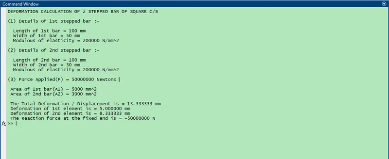
Image shows the 2 stepped bar arrangement before deformation
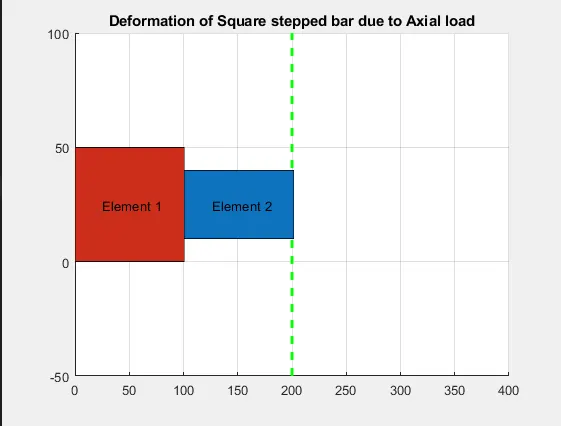
Image shows the deformation of the 2 stepped bars after the application of axail load.
Youtube Link-