Plotting Transient Motion of Simple Pendulum using MatLab

Aim:

To write a program in MatLab to simulate the motion of a simple pendulum using ODE.

Objective:

• Solve the ODE that represents motion of a simple pendulum.
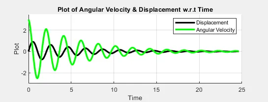
• Plot a graph to study the change in Angular Velocity and Displacement of the pendulum w.r.t to time.
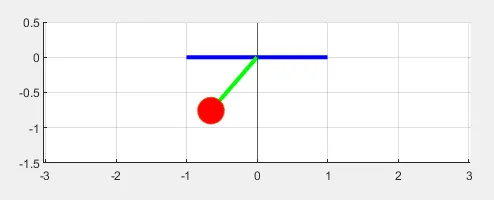
• Plot the figure of simple pendulum and animate to visualize its motion.

Theory:

In Engineering, ODE is used to describe the transient behavior of a system. A simple example is a pendulum.

Similarly, there are hundreds of ODEs that describe key phenomena and if you have the ability to solve these equations then you will be able to simulate any of these systems.

The way the pendulum moves depends on the Newtons second law. When this law is written down, we get a second order Ordinary Differential Equation that describes the position of the "ball" w.r.t time.

Governing Equation:

The second order differential equation is given by,

`------>(1)`

From the above equation,

• g = gravity in m/s2,
• L = length of the pendulum in m.
• m = mass of the ball in kg.
• b = damping coefficient.

Solution to the equation:-

Let

`theta = theta_1`

`(d theta)/dt = (d theta_1)/dt = theta_2`

`(d^2 theta)/dt^2=(d^2 theta_1)/dt^2=d/dt ( (d theta_1)/dt ) = (d theta_2)/dt`

Here we get the first equation of the 1st order ODE

`(d theta_1)/dt = theta_2 ----> (2)`

Now substitute `theta_1` and `(d theta_1)/dt` in equation (1)

we get,

`(d theta_2)/dt = -b/mtheta_2-g/lsintheta_1------>(3)`

Arranging equations 2 and 3 into matrix we get,

`d/dt[[theta_1] ,[theta_2]] = [[theta_2],[-b/mtheta_2-g/lsintheta_1]]`

Now we will be integrating this solution matrix to get the values of displacement and angular velocity.

EXPLANATION OF THE CODE:

Assuming l=1 metre, m=1 kg, b=0.35, g=9.81 m/s^2.

Matrix theta_0 stores the initial angular displacement and velocity.

t_span stores 500 time intervals from 0 seconds to 20 seconds.

ode45 is an inbuilt function in MATLAB to solve ODE. It calls a user defined function 'ode_func' and requires the inputs .

ode_func is a function to create a solution matrix from the 2 first order ODE.

ode45 returns angular displacement and angular velocity with respect to time.

't' matrix holds all the 500 time intervals within '0 to 20 seconds'.

'results' matrix holds all the 500 values of displacement and angular velocity both with respect to time.

Later, separate plot commands have been used to plot the displacement and angular velocity v/s time graph i.e. figure1.

We use animatedline command to plot and animate the lines of angular velocity and displacement.

Now, code under figure 1 simulate's the pendulum. One end of the pendulum is fixed. The other end moves according to the solution of the ODE we had solved.

A for loop has been used to calculate the position of the bob with respect to time. The loop continues upto the last time interval. The pendulum hinge is at the origin

The coordinates of the position of the bob i.e. x1 and y1 can be calculated using XData and YData

A plot command has been used to plot the solid fixed line.

Another plot command has been used to join the string from x0,y0 to x1,y1 and plot the marker.

Later all the figure windows have been captured into a M matrix.

Movie function has been used to create a movie

MatLab Program:

Code for function 'ode_func' :-

function [dtheta_dt] = ode_func(theta,b,g,l,m)
       theta1 = theta(1);
       theta2 = theta(2);
       dtheta1_dt = theta2;
       dtheta2_dt = -(b/m*l)*theta2-(g/l)*sin(theta1);
       dtheta_dt = [dtheta1_dt;dtheta2_dt];
end

Main Program :-

clear 
close all
clc

%========================Given Inputs ==============================

b = 0.35;
g = 9.81;
l = 1;
m = 1;

%==================== Initial Condition =======================

theta_0 = [0,3];

%==================== Time Points =============================

t_span = linspace(0,25,500);

%==================== Solve Ode ===============================

[t,results] = ode45(@(t,theta) ode_func(theta,b,g,l,m),t_span,theta_0)

%========= Displacement & Velocity plot w.r.t Time ============

a = results(:,1);
b = results(:,2);

figure(1)

ax1=subplot(2,1,1);
axis([0 25 -3 3.5]);

h1 = animatedline('Color','k',"LineWidth",2.5,"Parent",ax1);
h2 = animatedline('Color','g',"LineWidth",2.5,"Parent",ax1);
grid on

xlabel('Time')
ylabel('Plot')
title('Plot of Angular Velocity & Displacement w.r.t Time')
legend({'Displacement','Angular Velocity'})

%===================== Pendulum plots =========================
ax2=subplot(2,1,2);
axis([-2.5 2.5 -1.5 0.5]);
axis equal
grid on
xline(0);
hold on

plot(ax2,[-1,1],[0,0],'linewidth',3,'color','b');

x0 = 0;        %initial 'x' co-ordinate of pendulum string
y0 = 0;        %initial 'y' co-ordinate of pendulum string

x1 = 1*sin(results(:,1));   % 'x' co-ordinate where the bob is attached
y1 = -1*cos(results(:,1));  % 'y' co-ordinate where the bob is attached

l1=line(ax2,[x0 x1(1)],[y0 y1(1)],'linewidth',3,'color','g'); 
p=plot(ax2,x1(1),y1(1),'o',"MarkerSize",20,"MarkerFaceColor",'r');
hold off
%================== Animate plots in for loop =================

ct = 1;
for j = 1:length(t)
    
    % add points one at a time to dispacement/velocity plot
    addpoints(h1,t(j),a(j))
    addpoints(h2,t(j),b(j))
    
    % add points one at a time to pendulum plot
    p.XData=x1(j);
    p.YData=y1(j);
    
    % Animate the string
    l1.XData = [x0 x1(j)];
    l1.YData = [y0 y1(j)];
    drawnow;
    M(ct) = getframe(gcf);
    ct = ct+1;
    
end

%=================== Syntax for Movie =========================
movie(M)
vf = VideoWriter('simple_pendulum.mp4', 'MPEG-4')
open(vf)
writeVideo(vf,M)
close(vf)

Results:

Conclusion:-

• From the above graph we can conclude that the angular velocity and displacement of the pendulum gradually decreases w.r.t time.

Video of the plot :-

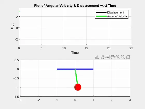
above video shows the transient motion of the pendulum and its corresponding variation in Angular velocity and displacement w.r.t time.

Youtube video link:-

https://youtu.be/gFggxFy8_7Q