Exhaust Port Challenge

OBJECTIVE:

• Setup a case of exhaust port conjugate heat transfer simulation and study the effect of mesh size on the results.
• Calculate the wall heat transfer coefficient on the internal solid surface
• Extract velocity and temperature contours
• Also, explain how to verify the results.

THEORY

Conjugate Heat Transfer

The exchange of thermal energy between two or more bodies is termed as Heat transfer and the rate of heat transfer is dependent on the temperature difference between them.

Conjugate heat transfer (CHT) is used to describe processes which involve variations of temperature within solids and fluids, due to thermal interaction between the solids and fluids. In solids, the conduction is the main mode of heat transfer whereas in liquid the convection is the main mode. The heat transfer depends on the heat transfer coefficient of each material and the temperature difference between the bodies.

The approach is used to design an efficient heat transfer application and optimizing them. Various applications of CHT is HVAC applications, car radiators, exhaust ports, heat sink, heat exchangers, etc.

PROCEDURE

The following procedure is followed in setting up the simulation and extracting the results.

Geometry

• import the geometry to SpaceClaim

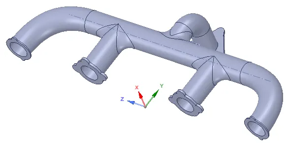
• create volume using edges

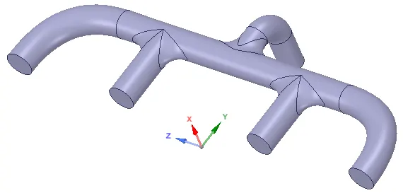
• create a shared topology using the share option to assign a common surface between the volume and the solid body and create a conformal mesh

Mesh

• In the first iteration create a mesh using the default value

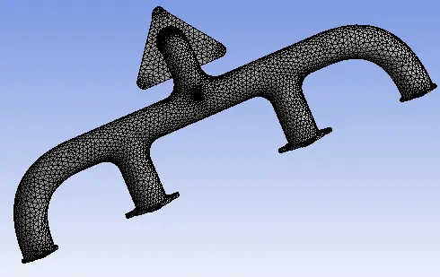
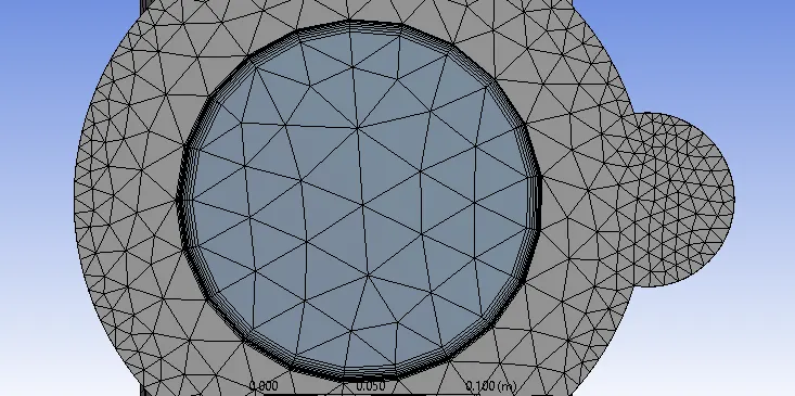
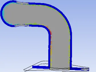
• As a part of mesh refinement create 5 inflation layers on the interior volume to capture better results near the interface. This thickness of the inflation layer depends on the value of Y+.

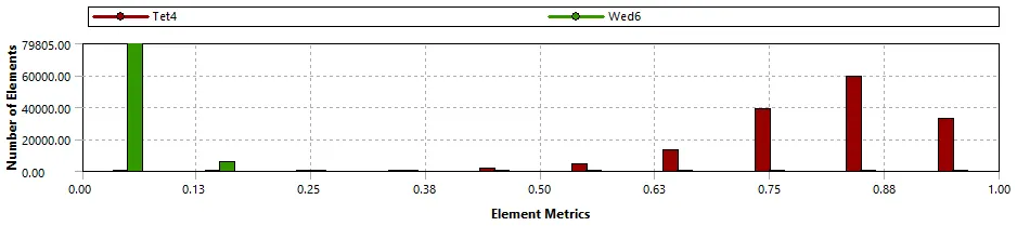
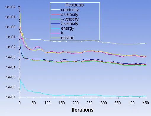
• Check for the acceptable mesh quality

Setting up Physics

• General -> Steady-state, pressure-based solver
• Model -> Energy equation -On, K epsilon model
• Boundary condition -> inlet = velocity = 5m/s and temperature 700 K
• Initialization -> Hybrid initialization to create initial condiitons inside the geometry.
• Create an animation for temperature contour variation (if required)
• Run Calculation

Results and Post Processing

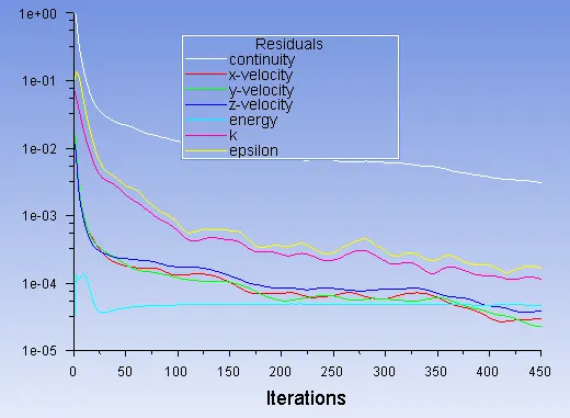
• Stop the solution once the convergence is reached.
• Contours - Pressure, Temperature, and velocity
• Streamline - velocity streamline
• Wall Heat transfer coefficient contour.

RESULTS & DISCUSSION

Case 1 - Baseline default mesh

Mesh quality

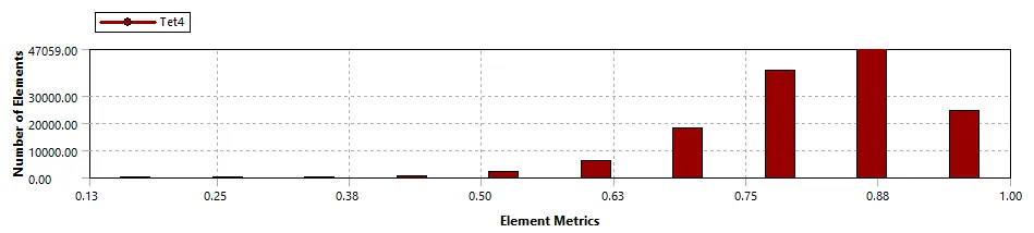
Nodes: 27247

Elements: 136855

Residual plots

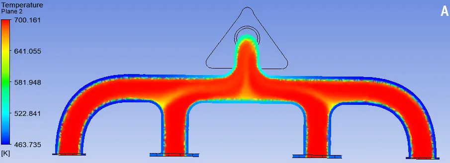
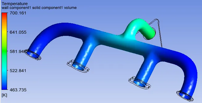
Temperature Contour

Flow temperature

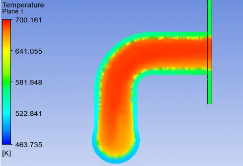
Wall Temperature

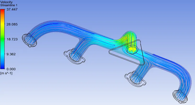
Velocity contour

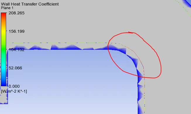
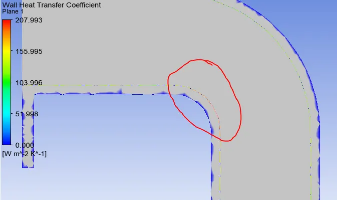
Wall Heat transfer coefficient contour

Case 2 - Refined Mesh 1, solid = 0.025m and inflation layer total thickness = 0.005m

Mesh quality

Nodes: 76025

Elements: 232836

Residual plots

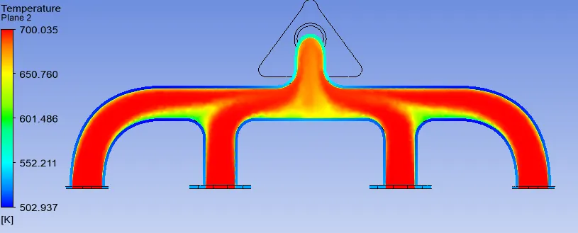
Temperature Contour

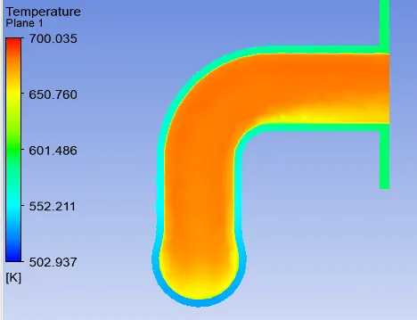
Flow Temperature

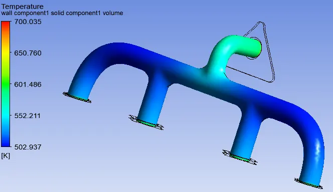
Wall Temperature

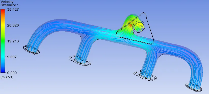
Velocity contour

Wall Heat transfer coefficient contour

Case 3 - Refined Mesh 2, solid = 0.01m and inflation layer total thickness = 0.005m

Mesh quality

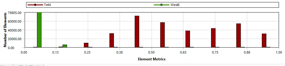
Nodes: 109944

Elements: 417289

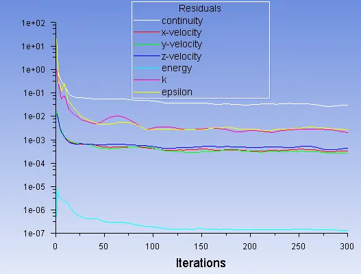
Residual plots

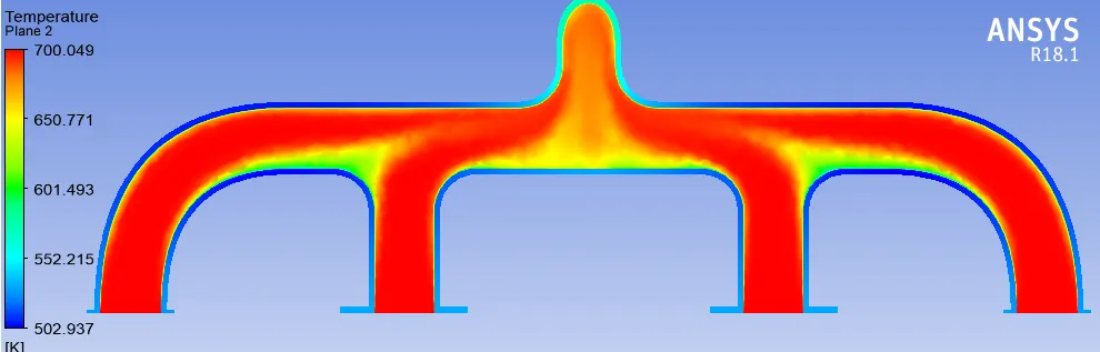
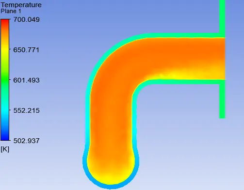
Temperature Contour

Flow Temperature

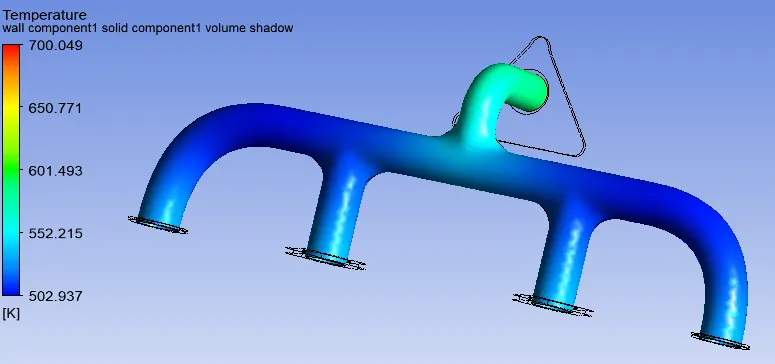
Wall Temperature

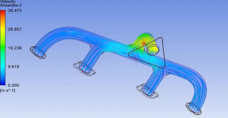
Velocity contour

Wall Heat transfer coefficient contour

Mesh	Nodes	Elements	Inlet velocity, m/s	Outlet Velocity, m/s	Inlet temperature, K	Outlet temperature, K	Max Wall Heat Transfer coefficient, W/(m2K).
default	27247	136855	5	25.310456	700	680.88485	65.719659
0.025m	76025	232836	5	25.204834	700	676.85945	191.28542
0.01m	109944	417289	5	25.208988	700	676.90131	191.31237

• With mesh refinement, we see a proper temperature distribution from inlet to outlet
• The outlet velocity is much more than the inlet velocity which is due to the law of mass conservation.
• In the temperature distribution contour in the wall, the wall temperature is higher where all flow converges as oppose to the individual inlet which is due to higher velocity of flow. Due to this, we observe a high value of HTC near the wall region where the flow converges.

How would you verify if the HTC predictions from the simulations are right? On what factors does the accuracy of the prediction depend on?

We can calculate the heat transfer coefficient using the following formula

h = (k_w/D_H)*Nu

where k_w is the thermal conductivity of the liquid, D_H is the Hydraulic diameter, and Nu is the Nusselt Number which is determined by the following equation:

Nu = 0.023Re^0.8Prⁿ

where Re is the Reynolds number: Re = (ρ * v * D_H)/(μ)

And Pr is the Prandtl number: Pr = (C_p* μ)/k_w

The prediction of HTC mainly depends on the following factors

• Properties of the fluid
• The velocity of flow as we can see the max HTC in the region where there is a maximum velocity
• Geometrical domain
• Mesh refinement (capturing the geometry, smaller element size, inflation layers)
• Topology sharing to create a conformal mesh and thereby having a correct heat transfer between the flow and the solid body.
• If there is external flow, then it also depends on that material and its convective heat transfer coefficient and flow velocity.