Detailed report of engine kinematics

Aim: Plot graph of compression and expansion in piston using engine kinematics.

Governing equation:

`V/V_c =1+1/2 〖(R+1-cosθ-(R^2-〖sin〗^2 θ)〗^(1/2)`

Here, V = Total volume,

Vc =Clearance volume,

R = 2 × (connecting rod/stroke),

θ = Revolution of crankshaft in degrees.

Objective of the project:

1. To make a new code in MATLAB using above equation.
2. Use this new code in as a function.
3. Apply this function in main code.

Body of content:

1. I used MATLAB software to run and perform this code.
2. The code is as given below,

clear all

close all

clc

 

% Inputs

gamma = 1.4

t3 = 2300  % in kelvin

 

% State variable

p1 = 101325

t1 = 500

 

% Engine geometric parameters

bore = 0.1;

stroke = 0.1;

con_rod = 0.15;

cr = 12;

 

% Calculating the swept volume and the clearance volume

 

v_swept = (pi/4) *bore^2*stroke;

v_clearence = v_swept/(cr-1);

 

v1 = v_swept + v_clearence

v2 = v_clearence

 

% State variables at state point 2

% p2v2^gamma = p1v1^gamma

% p2 = p1*(v1/v2) ^gamma = p1*cr^gamma

p2 = p1*cr^gamma;

 

%p1v1/t1 = p2v2/t2 | t2 = p2*v2*t1/(p1*v1)

t2 = p2*v2*t1/(p1*v1);

 

constant_c = p1*v1^gamma;

V_compression = engine_kinematics (bore, stroke, con_rod, cr,180,0);

 

P_compression = constant_c./V_compression. ^gamma;

 

% State variables at state point 3

v3 = v2

 

% p3v3/t3 = p2v2/t2| p3 = p2*t3/t2

p3 = p2*t3/t2

 

constant_c = p3*v3^gamma;

V_expansion = engine_kinematics (bore, stroke, con_rod, cr,0,180);

 

P_expansion = constant_c./V_expansion. ^gamma;

 

% State variables at state point 4

v4 = v1

 

%p3v3^gamma = p4v4^gamma | p4 = p3(v3/v4) ^gamma

p4 = p3*(v3/v4). ^gamma

 

 

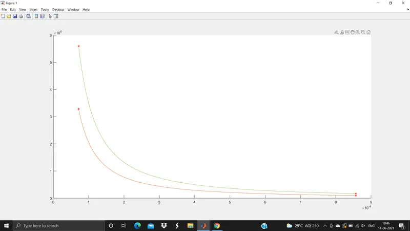
figure (1)

hold on

plot(v1, p1,'*','color','r')

plot(V_compression, P_compression)

plot(v2,p2,'*','color','r')

plot(v3,p3,'*','color','r')

plot(V_expansion, P_expansion)

plot(v4,p4,'*','color','r')

 

figure(2)

hold on

plot([v1 v2 v3 v4 v1],[p1 p2 p3 p4 p1],'color','b')

3. Also, I used a supplementary program (function) to make main program

Very clear and easy to understand.

4. The name of my supplementary program (function) is “engin_kinematics” and its code is given below.

function[V]=engine_kinematics(bore,stroke,con_rod,cr,start_crank,end_crank)

a = stroke/2;

R = con_rod/a;

v_s = pi/4*bore^2*stroke;

v_c = v_s/(cr-1);

theta = linspace(start_crank, end_crank, 100);

term1 = 0.5*(cr-1);

term2 = R+1-cosd(theta);

term3 = (R^2-sind(theta).^2).^0.5;

V = (1 + term1*(term2 - term3)).*v_c;

end

5. While making the function I give the same name to the function and the name of my file.

Conclusion:

1. Before using the function “engine_kinematics” the graph is a straight line.
2. But after applying the function it seems that the actual graph is not straight its curvilinear graph.