Week 4.1 - Genetic Algorithm

Title: Detailed report on Genetic Algorithm.

Aim: Using Genetic Algorithm optimize the value for given inputs.

Governing equations:

`f_(1.x)=[sin⁡(5.1πx+0.5) ]^6

f_(1.y)=[sin⁡(5.1πy+0.5) ]^6

f_(2.x)=exp⁡[4l n⁡(2) (x-0.0667)^2/(0.64)]

f_(2.y)=exp⁡[-4ln⁡(2)〖(y-0.0667)〗^2/(0.64)]`

Objective of the project:

1. Plot the 3D graph of the inputs.
2. Using optimization technique optimize the point at which the value of function is maximum.

Procedure:

1. Study the program in 3 ways.
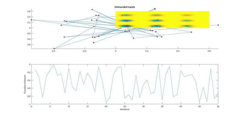
2. Study of statically behavior without upper and lower bounds.
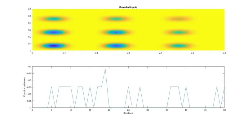
3. Study of statically behavior with upper and lower bounds.

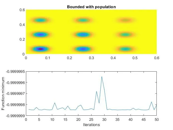
• Study of increasing GA iteration bounded with population.

2. Before writing a code there must be a create a function called stalagmite.
3. Code for the stalagmite function is given below,

function [F] = stalagmite(input_vector)

x = input_vector(1);

y = input_vector(2);

f1 = (sin((5.1*pi*x)+0.5))^6;

f2 = (sin((5.1*pi*y)+0.5))^6;

f3 = exp((-4*(log(2)*((x-0.0667)^2)/(0.64))));

f4 = exp((-4*(log(2)*((y-0.0667)^2)/(0.64))));

F = -1*f1*f2*f3*f4;

end

4. Optimize the inputs from stalagmite function using ga which is inbuild function of MATLAB.
5. The Entire code for the genetic algorithm is as follows,

clear all

close all

clc

x = linspace(0,0.6,150);

y = linspace(0,0.6,150);

num_cases = 50;

f = get_stalagmite(x,y);

% Study 1 - Statistical behavior

for i = 1:num_cases

[inputs, fopt(i)] = ga(@stalagmite,2);

xopt(i) = inputs(1);

yopt(i) = inputs(2);

end

figure(1)

subplot(2,1,1)

hold on

surfc(x,y,f)

shading interp

plot3(xopt,yopt,fopt,'marker','o','markersize',5,'markerfacecolor','r')

title('Unbounded inputs')

subplot(2,1,2)

plot(fopt)

xlabel('Iterations')

ylabel('Function minimum')

tic

% Study 2 - Statistical behavior - with upper and lower bounds

for i = 1:num_cases

[inputs, fopt(i)] = ga(@stalagmite,2,[],[],[],[],[0;0],[0.6;0.6]);

xopt(i) = inputs(1);

yopt(i) = inputs(2);

end

study2_time = toc;

figure(2)

subplot(2,1,1)

hold on

surfc(x, y, f)

shading interp

plot3(xopt,yopt,fopt,'marker','o','markersize',5,'markerfacecolor','r')

title('Bounded inputs')

subplot(2,1,2)

plot(fopt)

xlabel('Iterations')

ylabel('Function minimum')

% Study 3 increasing GA iterations

options = optimoptions('ga');

options = optimoptions(options,'PopulationSize',170);

tic

for i = 1:num_cases

[inputs, fopt(i)] = ga(@stalagmite,2,[],[],[],[],[0;0],[0.2,0.2],[],[],options);

xopt(i) = inputs(1);

yopt(i) = inputs(2);

end

study3_time = toc;

figure(3)

subplot(2,1,1)

hold on

surfc(x,y,f)

shading interp

plot3(xopt,yopt,fopt,'marker','o','markersize',5,'markerfacecolor','r')

title('Bounded with population')

subplot(2,1,2)

plot(fopt)

xlabel('Iterations')

ylabel('Function minimum')

Conclusion:

1. Optimization is a procedure which is executed iteratively by comparing various solution till an optimum or a satisfactory solution is found.
2. It is lengthy and difficult process to find best result using optimization for a human brain, but MATLAB works perfectly and accurately.