Curve fit using MATLAB
Aim
1) To write a code to fit a linear and cubic polynomial for the Cp data and plot the linear and cubic fit curves along with the raw data points
2) Use the split wise method to implement the program
Theory
What is a curve fit?
Curve fit helps us describe how our data changes mathematically and once we have a curve fit we can do additional mathematical operation which might not be possible in the initial set
Curve fitting is a process of constructing a curve which has the closet similarity for the series of data being considered. This method really helps in the mathematical modeling of an experiment on natural process
Concept of curve fit
Curve fitting is one of the most powerful and most widely used analysis tools in origin. Curve fitting examines the relationship between one or more predictors (independent variables) and a response variable (dependent variable), with the goal of defining a “best fit” model of the relationship
How to find a curve for a given data set and how to measure its goodness?
The curve fitting technique primarily focuses on creating equation from observed data points .The main methods to find the curve fit are
1) interpolation
2) curve fitting
Here we will be focusing on the 2nd part curve fitting because in interpolation if the data are repeating itself then when we plot them they form a clustered and that does not give a meaningful curve.
One of the most common techniques used to create the equation from data points is curve fit. In this, we will be finding a single equation which satisfies the entire range of data points
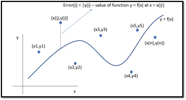
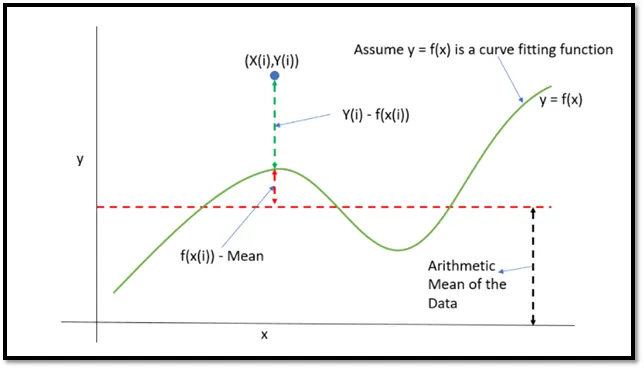
To choose the best curve fit we have to reduce the error which is shown in the graph and these errors are reduced by increasing the order of the polynomial but the user should also keep in mind that by increasing the order of the polynomial he should not get a condition of overfitting where it will completely give us the wrong data and interpretation of the curve after a certain point
The most common method is the least square method for finding a fitting function as long the function is a polynomial
The mathematical representation of error is

After finding the curve for the data points and checking whether it satisfies them or not, we then move on to check the goodness fit criteria of the curve/equation
The main four methods to check the best fit are
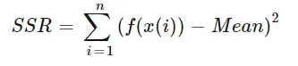
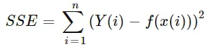
1) The sum of squares due to errors (SSE)


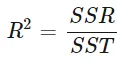
2) R-square
Basically what this values tells is that higher the value of r-square the better is the curve. This value of R-square ranges from 0-1.

3) Adjusted R-square
Adjusted R – square is basically as same as r-square but the only difference is that it doesn’t take into account the effects of the independent variable that has a very minimum effect in the contribution of the error in the curve.
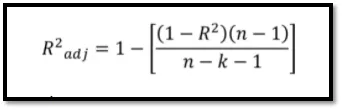
n - Number of data points
k - The number of independent variables
4) Root mean squared error (RMSE)
This is also known as fit standard error and the standard error of the regression. It is an estimate of the standard deviation of the random component in the data, and is defined as,
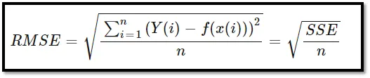
n - Number of data points
so in conclusion we can say that these 4 quantities can deduces the goodness of fit. The value of R-square is typically greater than 0.95 for a good curve fit
Code for cubic polynomial equation
clear all
close all
clc

%loading the data for the excecution of the program
cp_data=load('data');
temp = cp_data(:,1);
cp = cp_data(:,2);
%curve fit
%cp=a*x^3 + b*x^2 + cx + d

co_effs = polyfit(temp,cp,3);%this polyfit command actually makes the equation for set of datapoints we have and gives us the value for the coffient of the polynomial that we require.
predicted_cp = polyval(co_effs,temp);%finding the value of cp by using the polyval function where we use the values of cofficient of the function we found and temp


for i=length(cp)%using for loop to take into account all the value of 3200 data entry
    x(i) = (predicted_cp(i)-cp(i))^2;
    y(i) = (predicted_cp(i)-mean(cp))^2;
end
SEE = sum(x)% summing up all the values to find the sum of squares of regression
SRR = sum(y)% summing up all the values to find the sum of squared errors
R_sq = (SRR/(SRR+SEE))
k=0;%no of independent varibales
n=length(cp); %no of data points
adj_R_square = 1-(((1-R_sq)*(n-1))/(n-k-1))
RSME=sqrt(SEE/n)
if(R_sq>0.95) % running the if else condition to display weather the cruve is good or not. only displays when the r square value is greate
    disp('curve good')
else
    disp('curve bad')
end
%compare my curve fit with the original data and also labeling and plotting
%the data with proper legend
plot(temp,cp)
hold on
plot(temp,predicted_cp,'color','r')
xlabel('Temperature [K]')
ylabel('specific heat [KJ/Kmol-K]')
legend('original dataset','curve fit')
%plotting the graph between temperature and specific heat
grid on
Code for linear equation
clear all
close all
clc

%loading the data for the excecution of the program
cp_data=load('data');
temp = cp_data(:,1);
cp = cp_data(:,2);
%curve fit
%cp=a*x^3 + b*x^2 + cx + d

co_effs = polyfit(temp,cp,1);%this polyfit command actually makes the equation for set of datapoints we have and gives us the value for the coffient of the polynomial that we require.
predicted_cp = polyval(co_effs,temp);%finding the value of cp by using the polyval function where we use the values of cofficient of the function we found and temp


for i=length(cp)%using for loop to take into account all the value of 3200 data entry
    x(i) = (predicted_cp(i)-cp(i))^2;
    y(i) = (predicted_cp(i)-mean(cp))^2;
end
SEE = sum(x)% summing up all the values to find the sum of squares of regression
SRR = sum(y)% summing up all the values to find the sum of squared errors
R_sq = (SRR/(SRR+SEE))
k=0;%no of independent varibales
n=length(cp); %no of data points
adj_R_square = 1-(((1-R_sq)*(n-1))/(n-k-1))
RSME=sqrt(SEE/n)
if(R_sq>0.95) % running the if else condition to display weather the cruve is good or not. only displays when the r square value is greate
    disp('curve good')
else
    disp('curve bad')
end
%compare my curve fit with the original data and also labeling and plotting
%the data with proper legend
plot(temp,cp)
hold on
plot(temp,predicted_cp,'color','r')
xlabel('Temperature [K]')
ylabel('specific heat [KJ/Kmol-K]')
legend('original dataset','curve fit')
%plotting the graph between temperature and specific heat
grid on
Explanation of the code
1) We start our program with the usual command clear all, close all, clc which clears out all the previous data and variable which are if any sorted.
2) We then load the data of the values of temperature and specidic heat from the data file which must me in the same directory where we saved our program. To load the data from the data file we use the command load (‘data’) and store it in a variable which is called cp_data
3) temp = cp_data(:,1);
cp = cp_data(:,2);
This command stores the first column which are the values of temperature in the temp variable and the specific heat value in the cp variable and this only accesses the second column
3) We use the polyfit command to predict the curve for the given data set and thus from that extract the value of the coefficient. The num of the coefficient depends on the order of the polynomial. We store the value of the coefficient in the variable called co_effs.
4) since we are taking the value of temperature as our independent variable and the predicted cp is the dependent variable which is dependent on the changing value of temperature, we calculate that using the command polyval(co_effs,temp); .
5) now we have the value of temperature, preidicted value of specific heat for the cubic polynomial we have and the value of coefficient, we can plot the graph and compare it to the real graph which is given by the original data set but before that we should run a check on how good is the curve fit for the given case.
6) since we know that the error in the function curve depends from point to point, to examine all the points we run a for loop so that it can go from 0-3200 points and these value are stored in x(i) and y(i) which are SEE and SRR (sum of squares of regression sum of squared errors)
7) Summing up all the values of SEE and SRR using the sum function and then we calculate the R-square value which is given by the relation (R_sq = (SRR/ (SRR+SEE)))
8) Usual only the R-square value is sufficient to measure the good fit of the curve function but for the sake of learning we also calculate the rest of the parameters which are adjusted R-square value & RMSE
9) we use the if else function to show where the curve is a good fit or not giving the condition that the curve is only good If the R-square value is 0.95 above, the value 0.95 means that the curve is in resemblance with the original curve to the extent of 95 %
10) The last step is to plot the graph with suitable labels and compare the 2 graph which are given by the data set and the polynomial which is deduced by the matlab for the given data set
11) We again repeat the same function for the linear polynomial as we only change the order of the function to 1 and run the same thing for this bunch of code
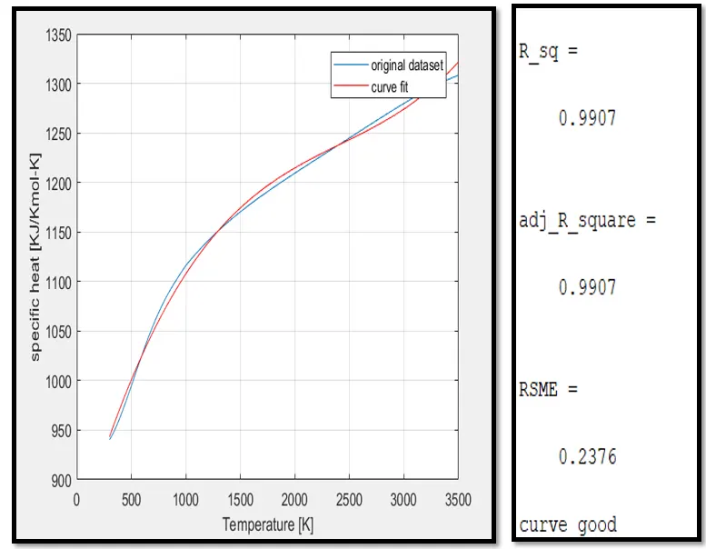
12) Comparing the curves and the values of R-Square, RMSE for both the curves we can see that as the polynomial order increases we get a curve that is closer and resembles the original data set curve and also the value of the R-Square value also increase from 0.9592 to 0.9902 which also indicates that the increasing the order of the polynomial gets us a good curve
Results
1) Linear polynomial
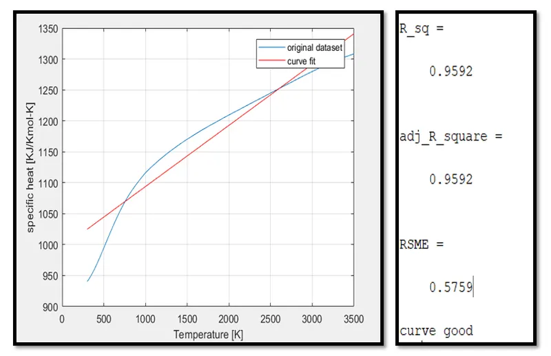
Cubic polynomial
Using Split wise function
%writing a code for curve fit via split wise method
clear all
close all
clc

%loading the data for the execution of the program
cp_data=load('data');
%dividing the temperature data into 5 sets
temp = cp_data(:,1);
temp1 = cp_data(1:640,1);
temp2 = cp_data(641:1281,1);
temp3 = cp_data(1282:1922,1);
temp4 = cp_data(1923:2563,1);
temp5 = cp_data(2564:3200,1);
%dividing the specific heat data into 5 sets
cp = cp_data(:,2);
cp1 = cp_data(1:640,2);
cp2 = cp_data(641:1281,2);
cp3 = cp_data(1282:1922,2);
cp4 = cp_data(1923:2563,2);
cp5 = cp_data(2564:3200,2);
%curve fit
%cp=a*x + b
%for the first segment of the data set from 1-640

co_effs_1 = polyfit(temp1,cp1,2);%this polyfit command actually makes the equation for set of datapoints we have and gives us the value for the coffient of the polynomial that we require.
predicted_cp_1 = polyval(co_effs_1,temp1);%finding the value of cp by using the polyval function where we use the values of cofficient of the function we found and temp

%for the first segment of the data set from 641-1281

co_effs_2 = polyfit(temp2,cp2,2);
predicted_cp_2 = polyval(co_effs_2,temp2);

%for the first segment of the data set from 1282-1922

co_effs_3 = polyfit(temp3,cp3,2);
predicted_cp_3 = polyval(co_effs_3,temp3);

%for the first segment of the data set from 1923-2563

co_effs_4 = polyfit(temp4,cp4,2);
predicted_cp_4 = polyval(co_effs_4,temp4);

%for the first segment of the data set from 2564-3200

co_effs_5 = polyfit(temp5,cp5,2);
predicted_cp_5 = polyval(co_effs_5,temp5);

%for the first set of data from 1-640

for i=length(cp1) %using for loop to take into account all the value of 640 data entry
    x5(i) = (predicted_cp_1(i)-cp1(i))^2;
    y5(i) = (predicted_cp_1(i)-mean(cp1))^2;
end
SEE1 = sum(x5)% summing up all the values to find the sum of squares of regression
SRR1 = sum(y5)% summing up all the values to find the sum of squared errors
R_sq1 = (SRR1/(SRR1+SEE1))
k=0;%no of independent varibales
n1=length(cp1); %no of data points
adj_R_square1 = 1-(((1-R_sq1)*(n1-1))/(n1-k-1))
RSME1=sqrt(SEE1/n1)
if(R_sq1>0.95) % running the if else condition to display weather the cruve is good or not. only displays when the r square value is greater than 0.95
    disp('curve good')
else
    disp('curve bad')
end

%for the first set of data from 641-1281

for i=length(cp2) %using for loop to take into account all the value of 640 data entry
    x2(i) = (predicted_cp_2(i)-cp2(i))^2;
    y2(i) = (predicted_cp_2(i)-mean(cp2))^2;
end
SEE2 = sum(x2)% summing up all the values to find the sum of squares of regression
SRR2 = sum(y2)% summing up all the values to find the sum of squared errors
R_sq2 = (SRR2/(SRR2+SEE2))
k=0;%no of independent varibales
n2=length(cp2); %no of data points
adj_R_square2 = 1-(((1-R_sq2)*(n2-1))/(n2-k-1))
RSME2=sqrt(SEE2/n2)
if(R_sq2>0.95) % running the if else condition to display weather the cruve is good or not. only displays when the r square value is greater than 0.95
    disp('curve good')
else
    disp('curve bad')
end

%for the first set of data from 1282-1922

for i=length(cp3) %using for loop to take into account all the value of 640 data entry
    x3(i) = (predicted_cp_3(i)-cp3(i))^2;
    y3(i) = (predicted_cp_3(i)-mean(cp3))^2;
end
SEE3 = sum(x3)% summing up all the values to find the sum of squares of regression
SRR3 = sum(y3)% summing up all the values to find the sum of squared errors
R_sq3 = (SRR3/(SRR3+SEE3))
k=0;%no of independent varibales
n3=length(cp3); %no of data points
adj_R_square33 = 1-(((1-R_sq3)*(n3-1))/(n3-k-1))
RSME3=sqrt(SEE3/n3)
if(R_sq3>0.95) % running the if else condition to display weather the cruve is good or not. only displays when the r square value is greater than 0.95
    disp('curve good')
else
    disp('curve bad')
end

%for the first set of data from 1923-2563

for i=length(cp4) %using for loop to take into account all the value of 640 data entry
    x4(i) = (predicted_cp_4(i)-cp4(i))^2;
    y4(i) = (predicted_cp_4(i)-mean(cp4))^2;
end
SEE4 = sum(x4)% summing up all the values to find the sum of squares of regression
SRR4 = sum(y4)% summing up all the values to find the sum of squared errors
R_sq4 = (SRR4/(SRR4+SEE4))
k=0;%no of independent varibales
n4=length(cp4); %no of data points
adj_R_square4 = 1-(((1-R_sq4)*(n4-1))/(n4-k-1))
RSME4=sqrt(SEE4/n4)
if(R_sq4>0.95) % running the if else condition to display weather the cruve is good or not. only displays when the r square value is greater than 0.95
    disp('curve good')
else
    disp('curve bad')
end

%for the first set of data from 2563-3200

for i=length(cp5) %using for loop to take into account all the value of 640 data entry
    x5(i) = (predicted_cp_5(i)-cp5(i))^2;
    y5(i) = (predicted_cp_5(i)-mean(cp5))^2;
end
SEE5 = sum(x5)% summing up all the values to find the sum of squares of regression
SRR5 = sum(y5)% summing up all the values to find the sum of squared errors
R_sq5 = (SRR5/(SRR5+SEE5))
k=0;%no of independent varibales
n5=length(cp5); %no of data points
adj_R_square5 = 1-(((1-R_sq5)*(n5-1))/(n5-k-1))
RSME5=sqrt(SEE5/n5)
if(R_sq4>0.95) % running the if else condition to display weather the cruve is good or not. only displays when the r square value is greater than 0.95
    disp('curve good')
else
    disp('curve bad')
end
n=length(cp);
total_see= (SEE1+SEE2+SEE3+SEE4+SEE5)/5
total_srr= (SRR1+SRR2+SRR3+SRR4+SRR5)/5
total_R_square = (total_srr/(total_srr+total_see))
total_RMSE = (total_see/n)

%compare my curve fit with the original data
plot(temp,cp);
hold on
plot(temp1,predicted_cp_1,'color','r')
hold on
plot(temp2,predicted_cp_2,'color','b')
hold on
plot(temp3,predicted_cp_3,'color','g')
hold on
plot(temp4,predicted_cp_4,'color','y')
hold on
plot(temp5,predicted_cp_5,'color','black')
xlabel('Temperature [K]')
ylabel('specific heat [KJ/Kmol-K]')
legend('original dataset','curve fit1','curve fit2','curve fit3','curve fit4','curve fit5')
%plotting the graph between temperature and specific heat
grid on
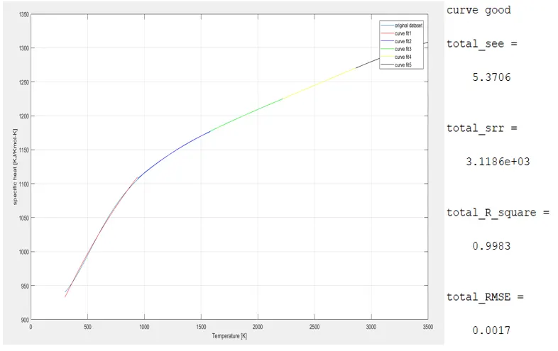
Result for split wise method with 2nd order polynomial
Conclusion
1) Comparing the curves and the values of R-Square, RMSE for both the curves we can see that as the polynomial order increases we get a curve that is closer and resembles the original data set curve and also the value of the R-Square value also increase from 0.9592 to 0.9902 which also indicates that the increasing the order of the polynomial gets us a good curve and concludes that the curve is a good fit.
2) From the split wise method we can see that a R-square value of 0.9983 is achieved which indicates that the split wise method is the most accurate method to get the best curve fit