Solving second order ODEs of a simple pendulum
Introduction
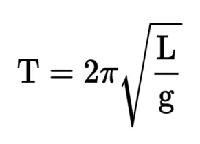
A simple pendulum is one which can be considered to be a point mass suspended from a string or rod of negligible mass. It is a resonant system with a single resonant frequency. For small amplitudes, the period of such a pendulum can be approximated by: Show. For pendulum length.
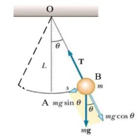
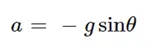
Acceleration of a pendulum
What is a differential equation?
A differential equation is any equation which contains derivatives, either ordinary derivatives or partial derivatives.
There is one differential equation that everybody probably knows, that is Newton’s Second Law of Motion. If an object of mass m is moving with acceleration and being acted on with force F then Newton’s Second Law tells us.
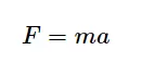
To see that this is in fact a differential equation we need to rewrite it a little. First, remember that we can rewrite the acceleration, a, in one of two ways.
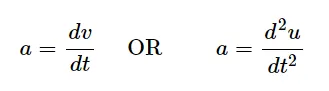
Where v is the velocity of the object and u is the position function of the object at any time t. We should also remember at this point that the force, FF may also be a function of time, velocity, and/or position.
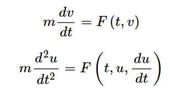
So, with all these things in mind Newton’s Second Law can now be written as a differential equation in terms of either the velocity, v, or the position, u, of the object as follows.
Ordinary differential equation
An ordinary differential equation (ODE) is an equation that involves some ordinary derivatives (as opposed to partial derivatives) of a function. Often, our goal is to solve an ODE, i.e., determine what function or functions satisfy the equation.
If you know what the derivative of a function is, how can you find the function itself? You need to find the antiderivative, i.e., you need to integrate.
The ODE at this moment in our case is the governing equation of the simple pendulum which is also based on newton’s second law of motion. It is a second order differential equation and we can identify this equation as second order by the order of the power the equation has
The mathematical expression of the second order ordinary differential equation is as follows
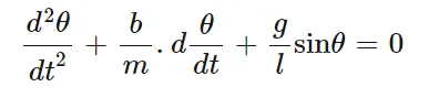
Where, b = damping coefficient
m = mass of the bob (Kg)
g = acceleration due to gravity (m/s^2)
l = length of the string m.
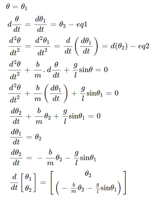
Theta 1 = displacement
Theta 2 = velocity
Theta 1 and theta 2 are the initial condition for the given problem
Given and assumption made in this problems are as follows:-
L=1meter
M=1kg
B=0.05
G=9.81m/s^2
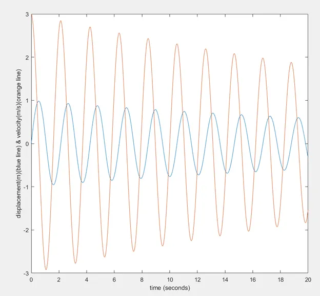
Simulating the motion between 0-20 seconds for angular displacement = 0, angular velocity = 3 rad/sec at time t=0.
MAIN CODE
clear all
close all
clc

%inputs
b = 0.05;
g = 9.81;
l = 1;
m=1;
ct=1;

%defining initial condition which are the displacement and velocity
theta_0 = [0;3];

%define the number of steps for the process
%defining the upper and the lower limit for the integration process
t_span = linspace(0,20,500);

%storing the outputs in t & results

[t, results] = ode45(@(t,theta) ishaan_func(t, theta,b,g,l,m),t_span, theta_0); %using ode45 because we have converted the 2nd order derivative into a first order derivate

%plotting the graphs showing the damping effects that shows with time
%vibration decrease
plot(t,results)

%labeling the x and y axis respectively
xlabel('time (seconds)')
ylabel('displacement(m)(blue line) & velocity((orange line)')

%for loop for to show the positon of every time step of pendulum

for i=1:length(results)
    t1=results(i)
    x0=0;
    y0=0;
    x1=l*sind(t1)%since it is oscillating along the x axis there for due to the geometry property we take the sin function at x1
    y1=-l*cosd(t1)
  figure(3)
  plot([1 -1],[0 0],'linewidth',5); % for the rigid wall support
  hold on%to show the previous plot of rigid wall support
  plot([x0 x1],[y0 y1],'color','r','linewidth',1)% for the oscillating string
  hold on%to show every time step of the oscillating string
  plot(x1,y1,'o','markers',30,'markerfacecolor','b')%for the representation of the oscillating ball
  hold off

   axis([ -0.2 0.2 -1.5 0.5])%defining the limits of the axis

    pause(0.01)% showing the next frame at every 0.01 secs
  H(ct)=getframe(gcf);%accumulating every frame and making an animation

    ct=ct+1;%incrementing the value as the loops takes the next step and thus capturing a new frame
end
movie(H)%creating a movie / animation
videofile = VideoWriter('pendulum.avi','uncompressed AVI');
open(videofile)
writeVideo(videofile,H)
close(videofile)
FUNCTION CODE
function [dthet_dt] = ishaan_func(t,theta,b,g,l,m)

theta1 = theta(1);% take fist value of theta which corresponds to the displacement
theta2 = theta(2);% take the second value of theta which corresponds to the velocity
dthet1_dt = theta2;
dthet2_dt= -(b/m)*theta2 - (g/l)*sin(theta1);
dthet_dt = [dthet1_dt; dthet2_dt];
end
RESULTS
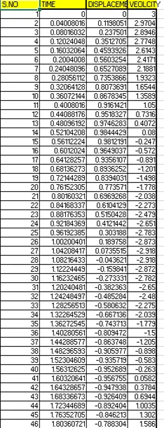
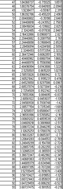
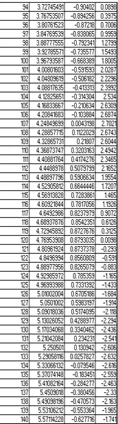
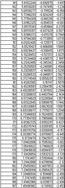
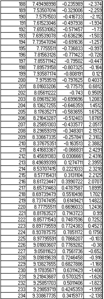
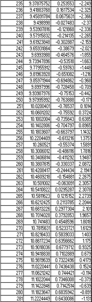
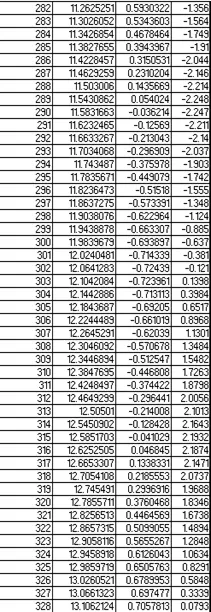
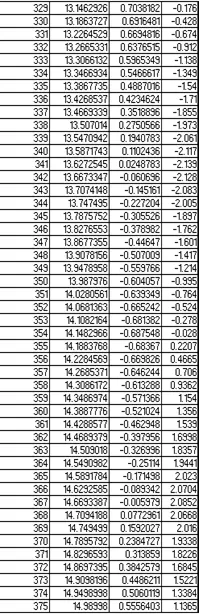
These are the data which represent the time and the location of the pendulum with respect to the time
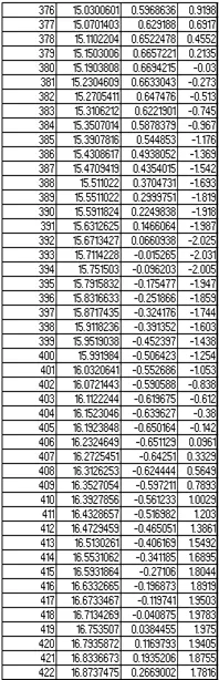
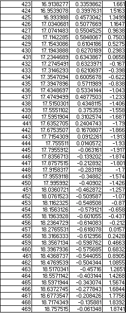
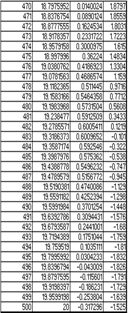
Graph
This graph plots the time vs displacement and time vs velocity for the second order ordinary differential equation which governs the motion of the simple pendulum and gives us the location of the pendulum (angular dispalcement) and its veloctiy at that postion with respect to that instantaeoes time. This graph is plotted for 500 points with respect to time where the lower limit is 0 and the upper limit is 20.
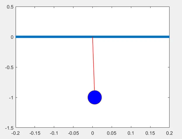
Link for animation
Please follow this link to see the animation of the simple pendulum which is created via matlab