Conjugate Heat Transfer Simulation
Aim:
The major objective of this project was to Simulate an Aluminium cylindrical tube for the Conjugate Heat Transfer problem using Converge CFD and Post-processing the result using ParaView to study the change of result when the major parameter is changed like grid size.
Introduction
The report contains a detailed description of the Conjugate Heat Transfer problem using converge CFD software, solving it using CYGWIN, and post-processing the result using ParaView. Various steps are discussed in this report while making a case set up for this case study. This report contains a detailed description of the case study with grid sizing, line plots, the effect of Superheating parameter, and contours.
Conjugate Heat Transfer (CHT) is when heat transfer occurs simultaneously within and between fluid and solid regions.
-The predominant mode of heat transfer in a fluid is convection.
-The predominant mode of heat transfer in a Solid is conduction.
Converge solves the fluid heat transfer using the energy equation.
converge solve the solid heat equation using the solid heat equation.
CHT Modeling Setup
There are several steps to setting up a CHT simulation
1.Define fluid and solid material and their physical properties
2.Configure the fluid and solid regions
3. Assign region to streams.
4. Use appropriate boundary conditions for the boundaries that separated different regions.
5. Select the time control method.
6. Set up post-processing.
Super-cycling
Super-cycling is a method used by CONVERGE Studio in the case of conjugate heat transfer problems with solid and liquid regions.
The integral problem here is that both solvers cannot run at the same speed since solving in the fluid domain is much faster owing to the time scale difference for heat transfer in liquids as compared to solids. This causes problems during the solution given that the solid side solver would not have reached a steady-state/convergence in the time the liquid solver does. This is where the concept of super-cycling can be used.
The basic idea of super-cycling is that the solver for the fluid domain is paused until the solver for the solid domain converges.
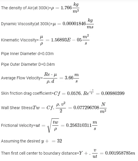
Calculation of Grid Size
Reynolds Number Re=7000
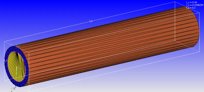
Geometry Creation
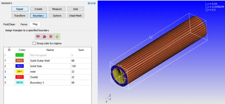
Boundary Creation
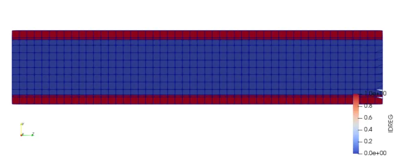
Simulation Result
Grid Dependence Test
Case Study 1: Mesh Size 0.004m
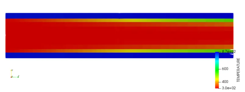
Temperature Contour
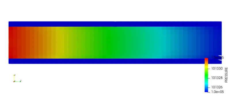
Pressure Contour
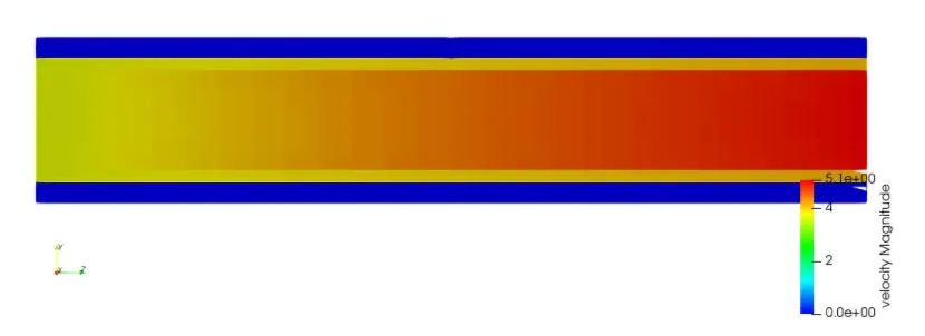
Velocity Contour
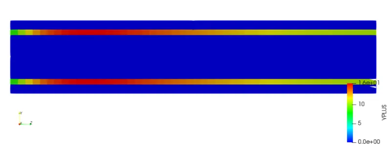
Y Plus Contour
Temperature Plot
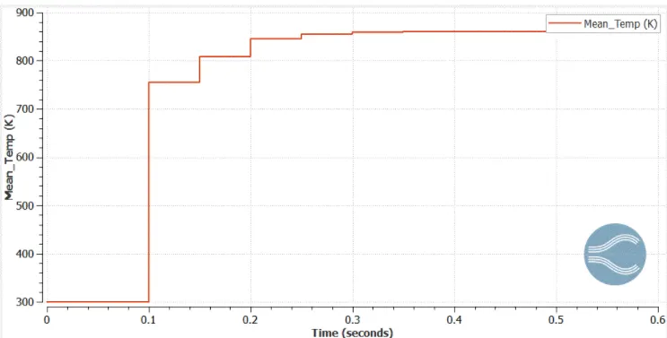
Inferences from the above contours:
- The temperature of the fluid increases near the boundary as it is in contact with the pipe. The same is shown in the animation as the simulation progresses.
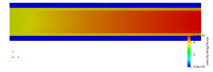
- The velocity contour shows the boundary layer formation in the flow thro' the pipe, though it does not give a clear picture as the mesh size is big.
- As usual there is a decreasing trend in the pressure as the flow propagates from higher pressure to lower pressure.
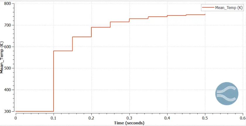
- The comparison of temperature convergence is presented in the last part of this section.
- Note:
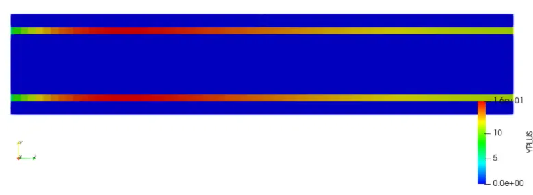
- The Y+ value is a dimensionless parameter used to determine which wall function has to be used and when, in order to predict the nature and behaviour of the fluid near the wall, i.e., the boundary. If it is less than 10, it is in the viscous sub-layer, if it is more than 30, it is turbulent, if it is in between then it is in the transition, which is undersirable.
- It also helps in determining the base grid and other parameters.
- Inference:
- The Y+ value is higher in places near the start of the flow, in the order of 14, which implies that it is in the transition phase.
- Basically, this value has minor significance for CHT simulation.
Case Study 2: Mesh Size 0.003m
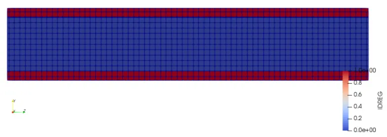
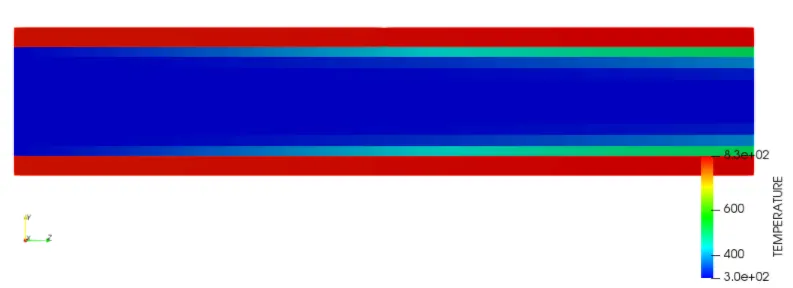
Temperature Contour
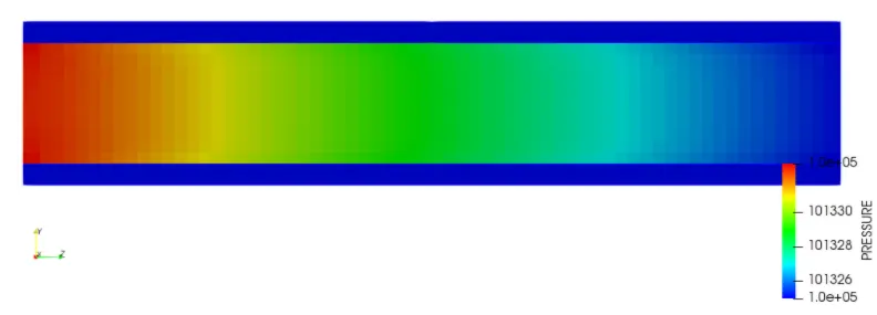
Pressure Contour
Velocity Contour
Y Plus Contour
Temperature Plot
Inferences from the above contours:
- Similarly, the temperature of the fluid increases near the boundary, but the variation in temperature along the diameter of the pipe could be seen with clarity as the mesh size is less as compared to the previous case. The same is shown in the animation as the simulation progresses.
- The boundary layer formation in the flow thro' the pipe could be witnessed in greater detail, which is accounted for the same reason.
- Similarly, there is a decreasing trend in the pressure.
- Inference:
- The Y+ value is higher in places near the start of the flow, in the order of 12, which implies that it is in the transition phase. Here, it is even more precise as the mesh size is reduced.
- This value has minor significance for CHT simulation.
Case Study 3: Mesh Size 0.002m
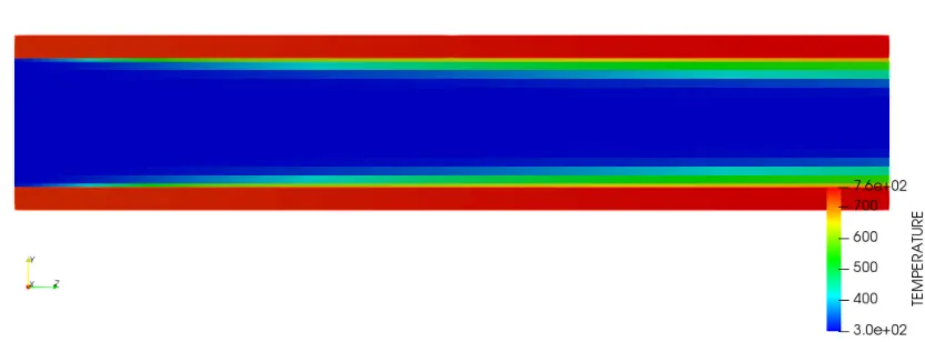
Temperature Contour
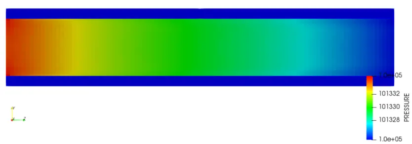
Pressure Contour
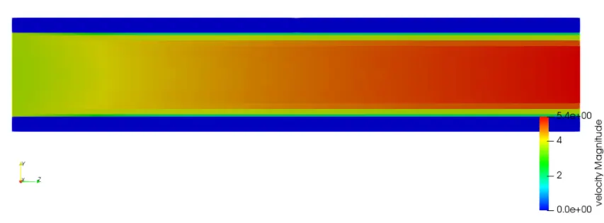
Velocity Contour
Y Plus Contour

Temperature Plot
Inferences from the above contours:
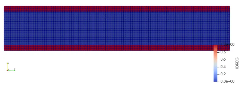
- Similarly, the temperature of the fluid increases near the boundary. It is clear that as the flow propagates thro, the pipe the temperature of fluid near the boundary increases and the influence of the heat supplied on the particles in the boundary increases along the length and it transfers along the diameter, which is depicted with clarity. The same is shown in the animation as the simulation progresses. This is dedicated to the mesh size, as it is the least in this case.
- The boundary layer formation is witnessed in even greater detail, the above reason applies for here too.
- Similarly, there is a decreasing trend in the pressure.
- Inference:
- The Y+ value is higher in places near the start of the flow, in the order of 8.2, which implies that it is in the viscous sub-layer.
- Basically, this value has minor significance for CHT simulation.
The links of Youtube videos are as follows-
Conclusion
Grid Dependency Test
1. When the grid size is being decreased the mesh size gets finer and Y+ range for lowest mesh also decreases
Y+ for 2mm grid Ranges from 0 to 7.3
Y+ for 3mm grid Ranges from 0 to 16
Y+ for 4mm grid Ranges from 0 to 16
2. As we decrease the mesh size there is also drop-in solid region temperature
The temperature for the 2mm grid is 850K Approx.
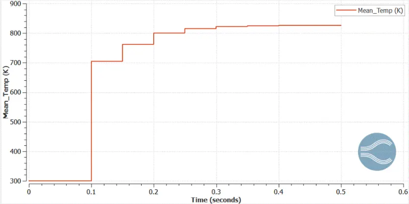
The temperature for the 3mm grid is 825K Approx.
The temperature for the 4mm grid is 750K Approx.
3. As we decrease the mesh the flow is viscous layer close to the wall and is more accurately captured.
Effect of Supercycle Stage Interval
Smaller the value of the supercycle stage the result is achieved faster because the simulation time is less.
Time for Supercycle Statge interval of 0.01 is about 0.18s and simulation time is 1668s
Time for Supercycle Statge interval of 0.02 is about 0.23s and simulation time is 1948s
Time for Supercycle Statge interval of 0.03 is about 0.30s and simulation time is 2166s