Conjugate Heat Transfer Analysis on a graphics card.
AIM: To perform a steady-state conjugate heat transfer analysis on a model of a graphics card.
Theory:
Conjugate Heat Transfer:
The Conjugate Heat Transfer (CHT) analysis type allows for the simulation of heat transfer between solid and fluid domains by exchanging thermal energy at the interfaces between them.
Conjugate heat transfer corresponds with the combination of heat transfer in solids and heat transfer in fluids. In solids, conduction often dominates whereas in fluids, convection usually dominates. Efficiently combining heat transfer in fluids and solids is the key to designing effective coolers, heaters, or heat exchangers. Forced convection is the most common way to achieve high heat transfer rate. In some applications, the performances are further improved by combining convection with phase change (for example liquid water to vapor phase change).
Heat transfer in solids and heat transfer in fluids are combined in the majority of applications. This is because fluids flow around solids or between solid walls, and because solids are usually immersed in a fluid.
Solving of CHT analysis of Graphic Card:
CASE-1:
Coarse Mesh
Geometry:
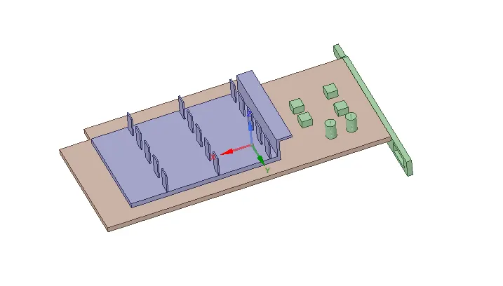
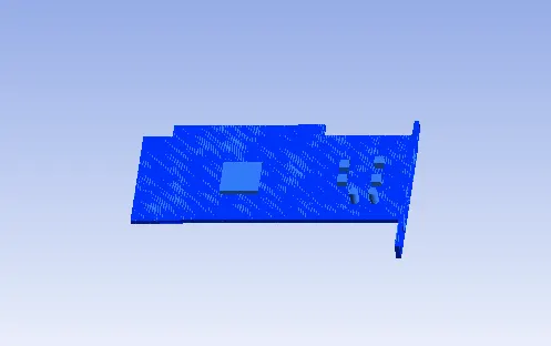
The graphic card used in this simulation is mentioned below which analysed in a closed enclose
Mesh:
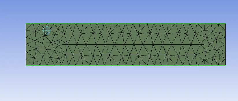
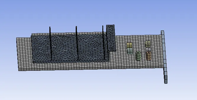
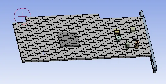
Coarse Mesh is used in this case and mesh details are shown below.
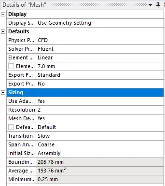

For Board, Processor and fins = 1mm element size. and body sizing is applied.
Setup & Solution:
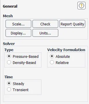
Pressure based solver and steady state conditions is applied.
Energy is enabled
K-Omega/SST model is used
Materials Used:
board = steel (density = 8030kg/m^3, Cp = 502.48j/kg-k, Thermal conductivity = 16.27w/m-k)
fins = copper (density = 8978030kg/m^3, Cp = 381j/kg-k, Thermal conductivity = 387.6w/m-k)
processor = nickel and source term enabled. (density = 8900kg/m^3, Cp = 460.6j/kg-k, Thermal conductivity = 91.74w/m-k)

inlet velocity 5m/s and temperature is 300K
Results and Discussion:
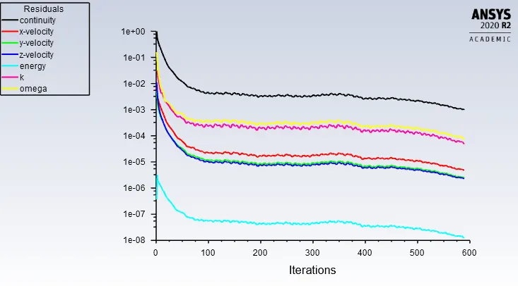
Residual Plot
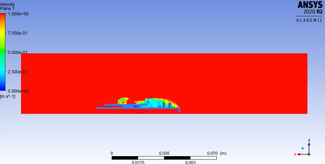
Velocity Contour
at 1m/s
at 3m/s
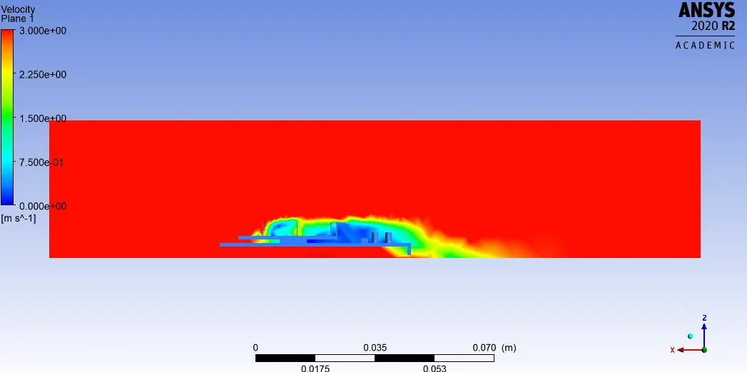
at 5m/s
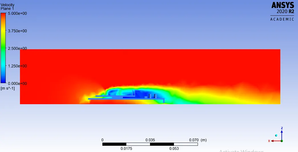
We can see the change in velocity around the
Temperature contour
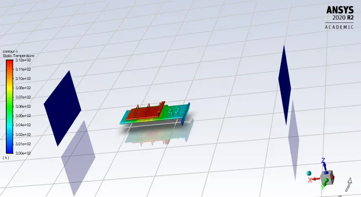
The maximum Temperature generated is 311.962K
Global Range
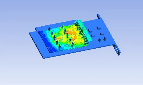
above, we can see that the 1st line of fins are cooler than the last line of fins.
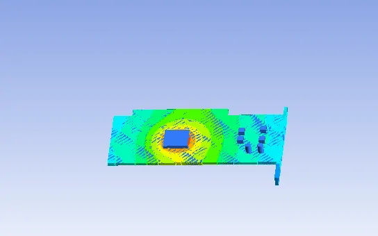
Local range temperature contour
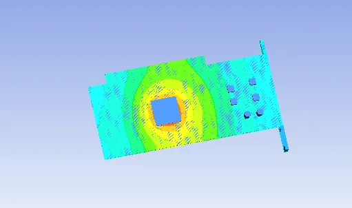
we can see heat distribution from processor.
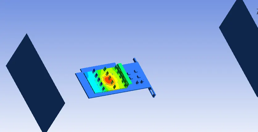
Wall Heat Transfer Coefficient:
The HTC generated is 407.343W/((m^2)*(K^(-1)))
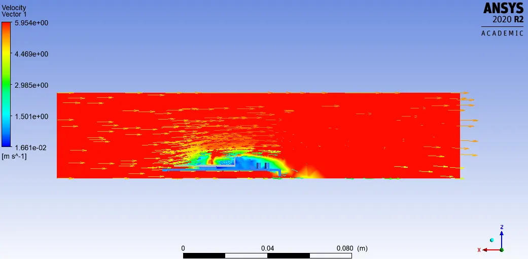
Velocity Vector
Three circulation regions are formed and their velocity is 0.01m/s
CASE-2:
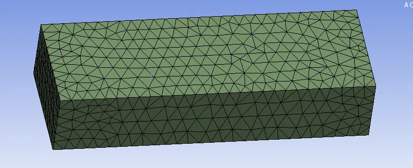
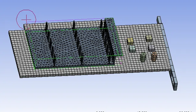
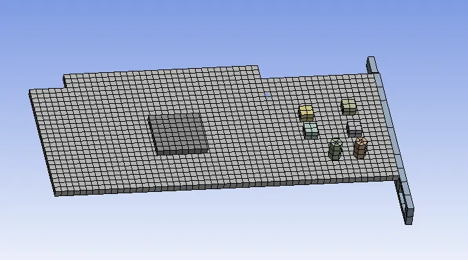
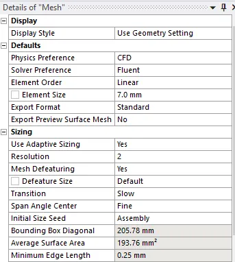
Refined Mesh
Mesh:
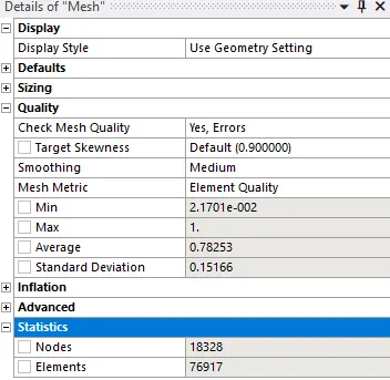
Setup Solution:
The settingup of solution is same as for Coarse case.
Materials used is same.
Results & Discussion:
Residuals plot:
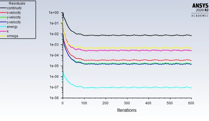
Velocity Contour:
at 1m/s
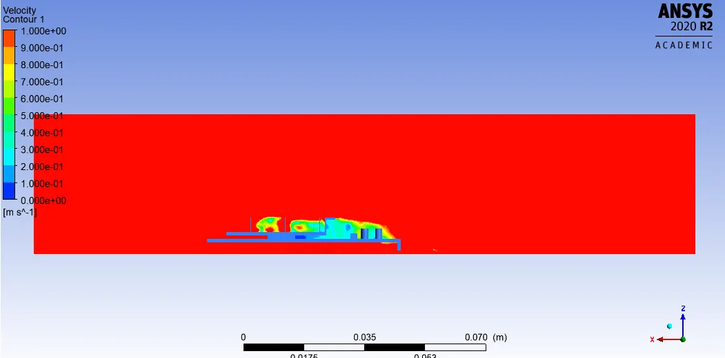
at 3m/s
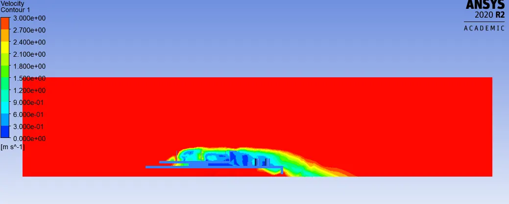
at 5m/s
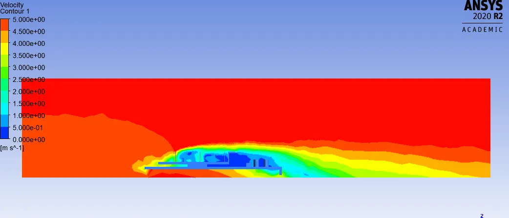
Temperature Contour:
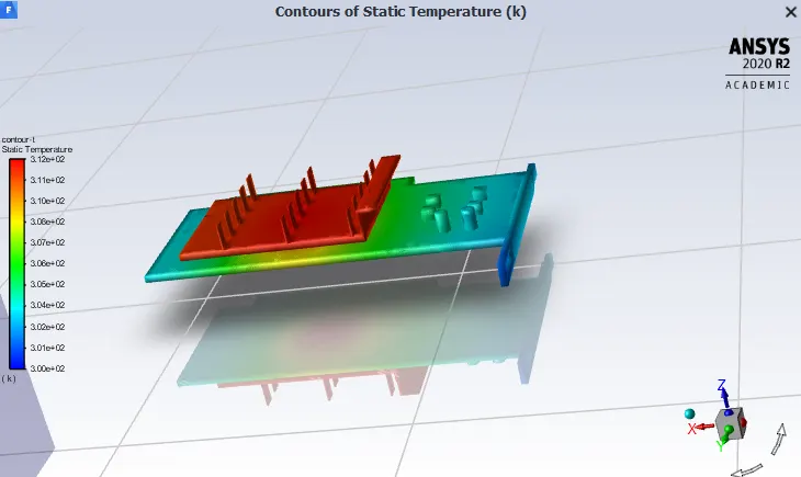
Temperature Global range at enclosure
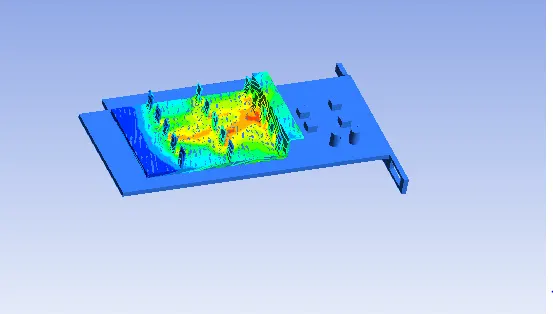
Heat distribution-processor
The maximum temperature generated is 311.962K
Wall Heat Transfer Coefficient:
The HTC generated is 484.924W/((m^2)*(K^(-1)))
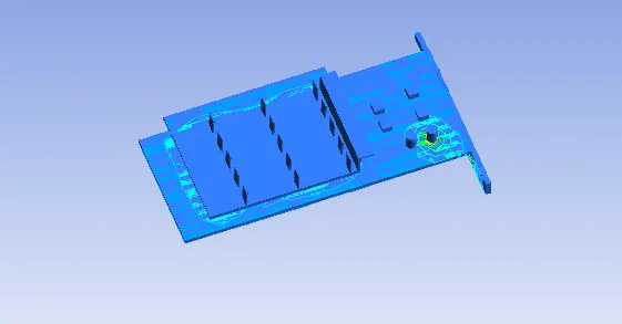
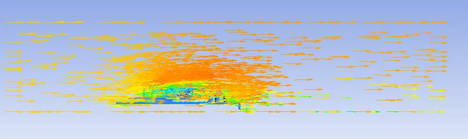
Velocity Vector:
| Mesh | Maximum Temperature | HTC |
| Case-1(Coarse) | 311.962K | 407.343 |
| Case-2(Refined) | 311.962K | 484.924 |
Conclusion:
From Coarse to Refined
Mesh tempetarure is same but the Heat Transfer Coefficient is increased.
Velocity distribution is clear in refined case.