Challenge on Combustion
OBJECTIVE:
Setup a case of combustion simulation on combustor model with methane-air as fuel and observe the mass fraction of different species and NOx and soot formation for the following 2 cases.
Case 1 - Perform regular combustion simulation with Methane-air-2 step mixture and plot the mass fraction of different species at different locations on combustor as shown below.
Case 2 - Perform a parametric study by adding water to fuel in proportion from 5% to 30% and plot the same results as discussed above and observe its effect.
Based on the results provide the necessary inferences.
PROCEDURE:
The reaction of the combustion for this simulation is

From the above equation, we can say that a = 1, b = 4, ar = 2
Thus calculating the mass fraction o each element, we get the mass fraction of fuel = 1, O2 = 0.23. This is used in defining the inlet boundary condition in subsequent steps.
Step 1 - Setting up the geometry
- Here we have a whole geometry of a combustor in 3D. For the simplification of the problem, we will deal with a 2D axisymmetric case.
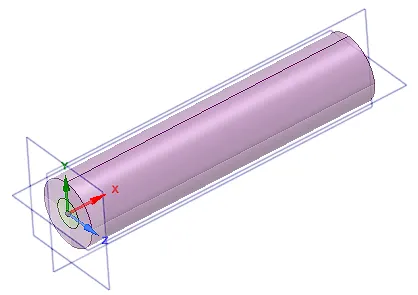
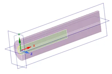
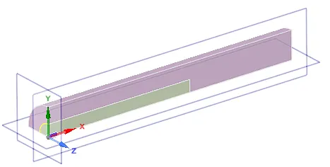
- For this, we need to convert the geometry to a 2D surface. Make sure that the axis of symmetry is X-axis and the geometry lies in the X-Y plane.

Step 2 - Meshing
- Here we need a fine mesh near the fuel inlet region so turn on proximity and curvature options.
- Select method -> triangles for tria elements.

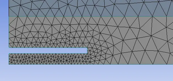
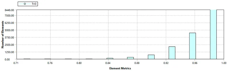
- Check the mesh quality
- Provide named selection.

Step 3 - Setting up the physics
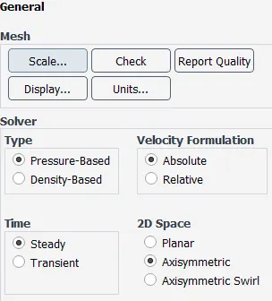
- Solver -> Steady-state, pressure-based, Axisymmetric
- Model -> Turbulence model - K epsilon -> Standard
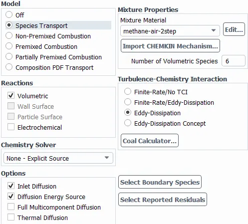
- Model -> species -> Volumetric -> inlet diffusion -> Diffusion energy source -> Mixture material = methane-air-2 step -> eddy dissipation model
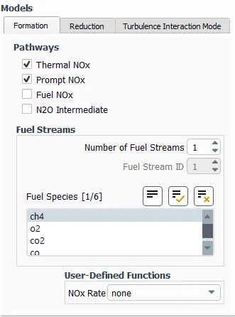
- Model -> species -> NOx model -> Thermal Nox -> Prompt NOx
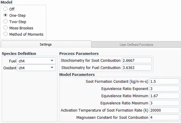
- Model -> Species -> Soot model -> One step soot model
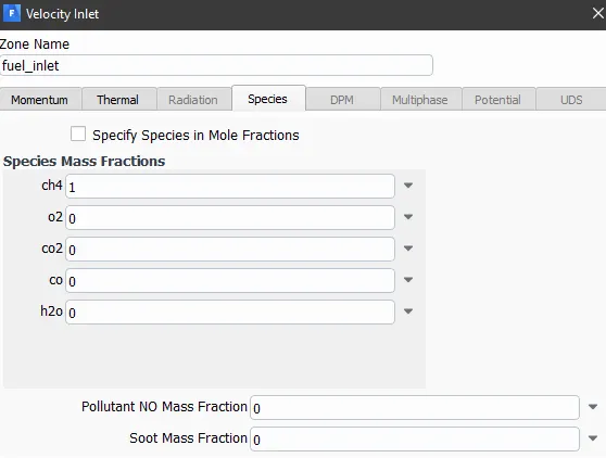
- Boundary conditions -> Fuel inlet -> velcotiy = 80m/s -> temperature = 300 K -> Species -> Mass fraction CH4 = 1
- Boundary conditions -> Fuel inlet -> velcotiy = 0.5m/s -> temperature = 300 K -> Species -> Mass fraction O2 = 0.23
- Boundary conditions -> Outlet -> pressure = 0
In setting up the physics for case 2, make the following changes in Boundary condition -> Fuel inlet
| CH4 | H2O | |
| Case 1 | 1 | 0 |
| Case 2a | 0.95 | 0.05 |
| Case 2b | 0.9 | 0.1 |
| Case 2c | 0.8 | 0.2 |
| Case 2d | 0.7 | 0.3 |
Step 4 - Initialization, Run calculation
- Hybrid initialization.
- enter no of iterations, run the calculation. wait for convergence.
Step 5 - Results
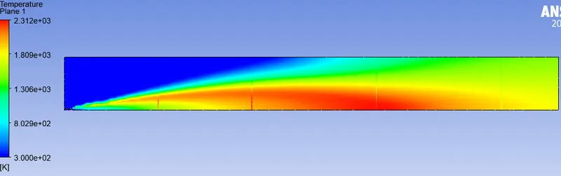
- Temperature and mass fraction contours were plotted
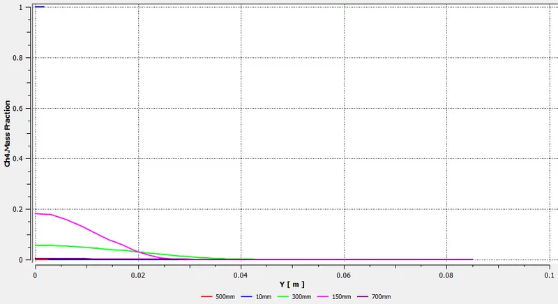
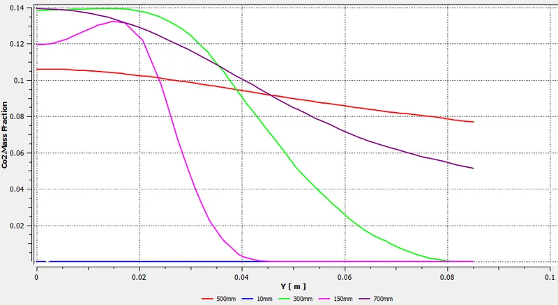
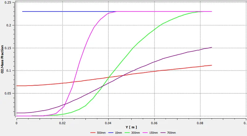
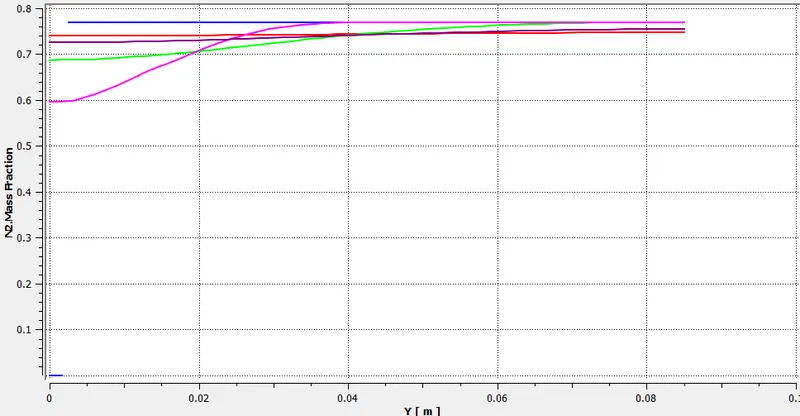
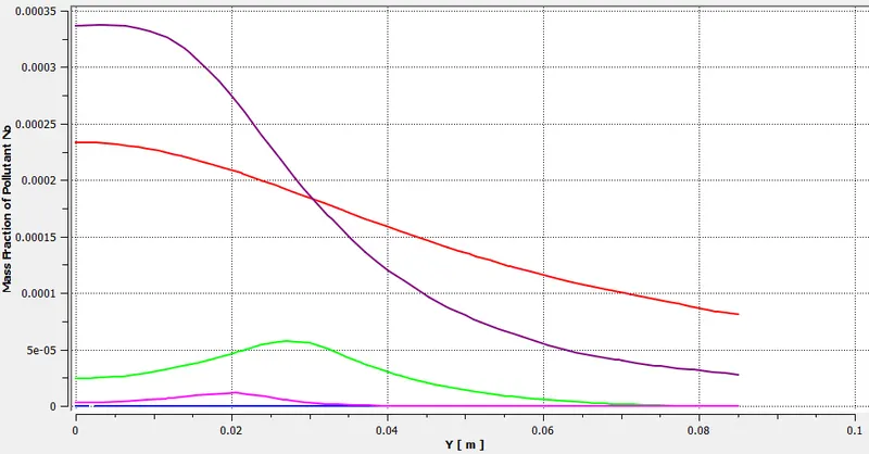
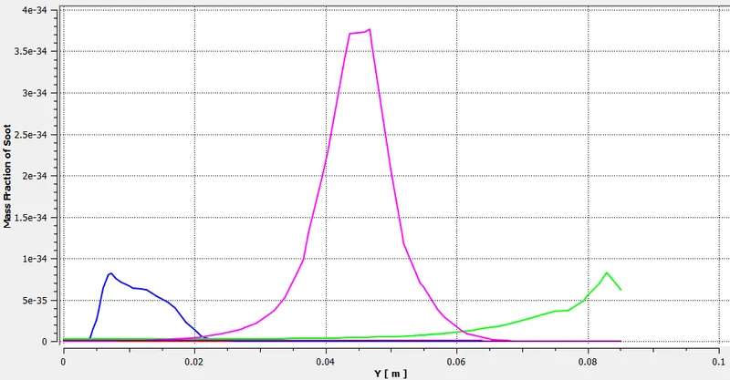
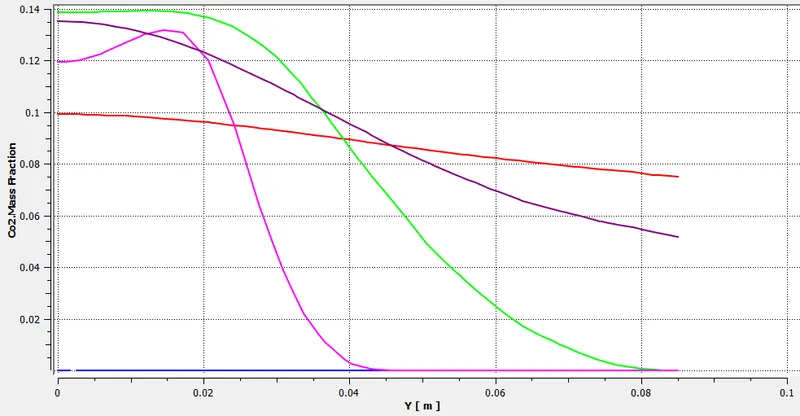
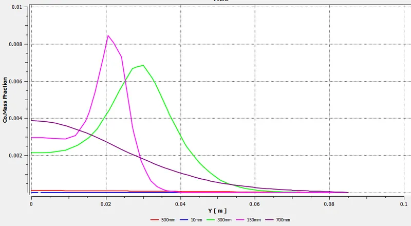
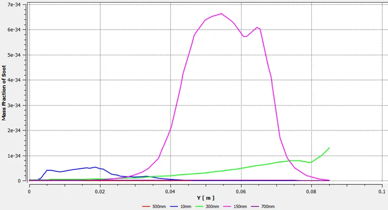
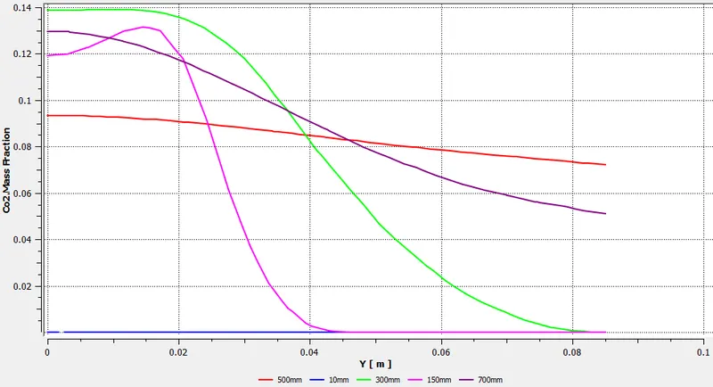
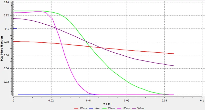
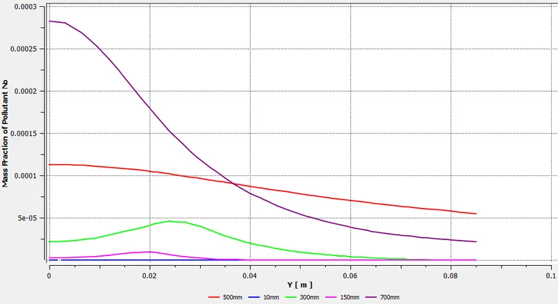
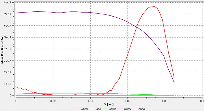
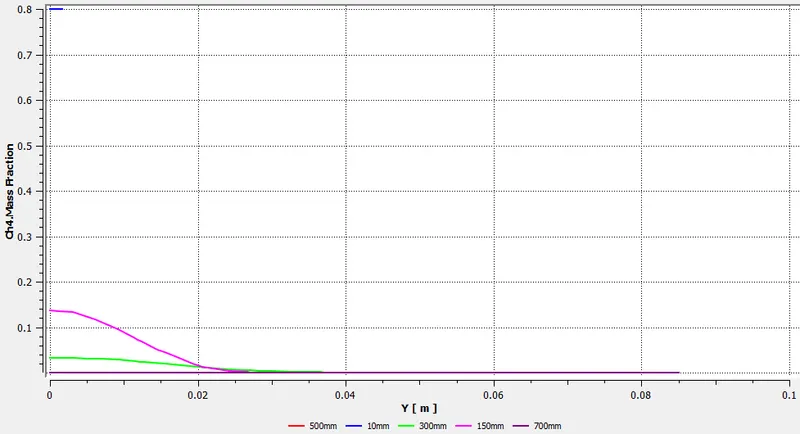
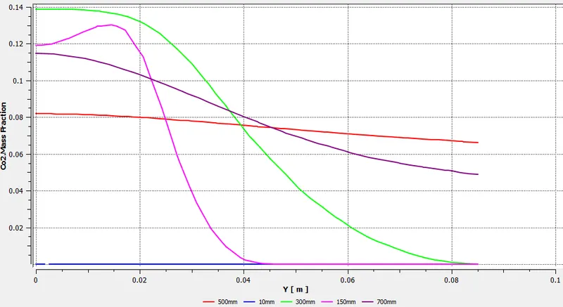
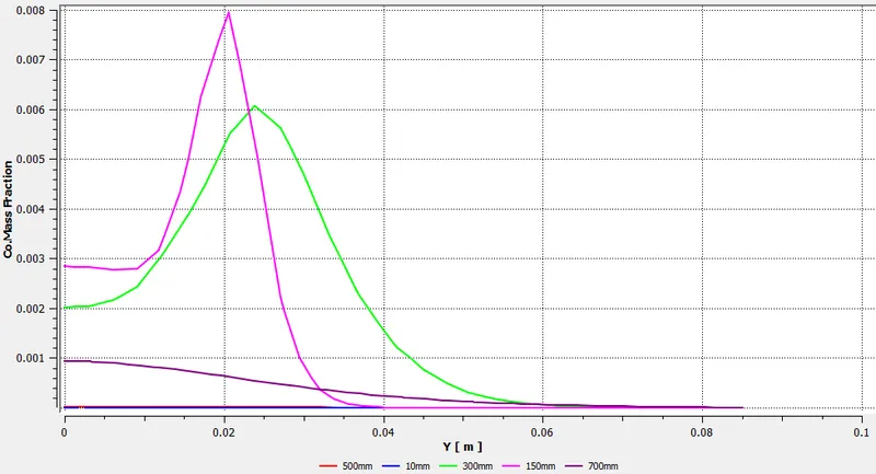
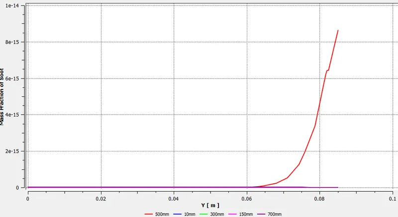
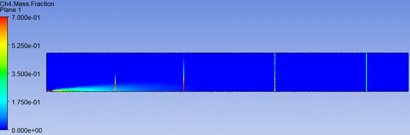
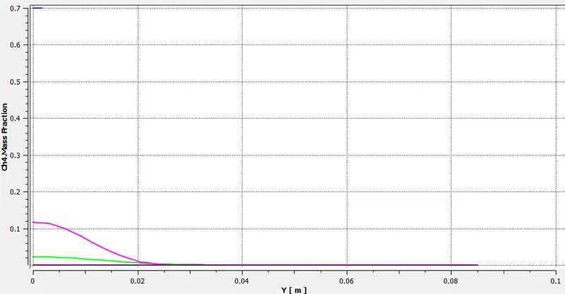
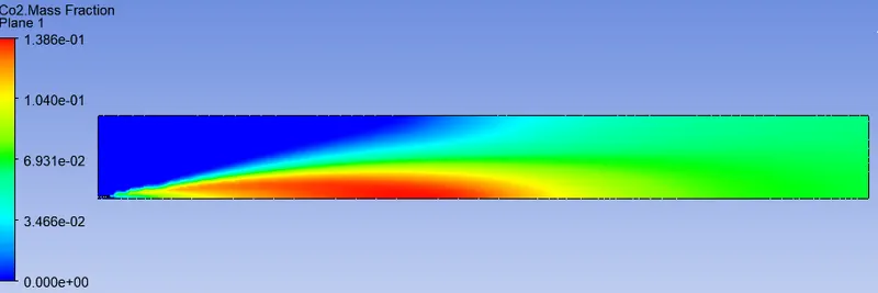
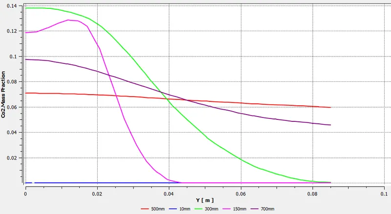
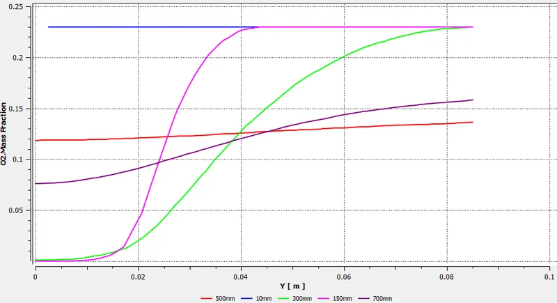
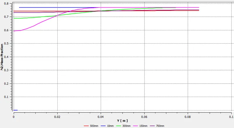
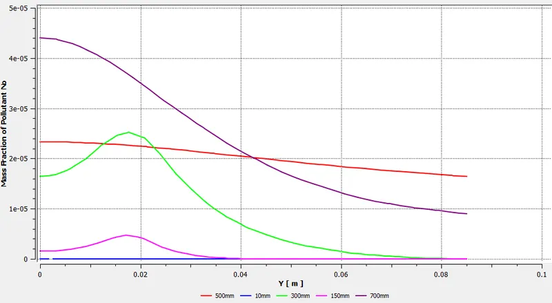
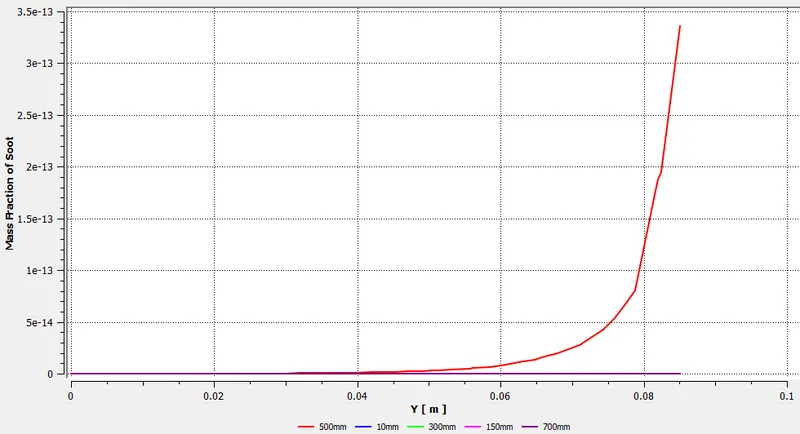
- Also, line plots at the different locations were plotted. At distance x = 10 mm, 150mm, 300mm, 500mm, 700mm

RESULTS
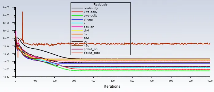
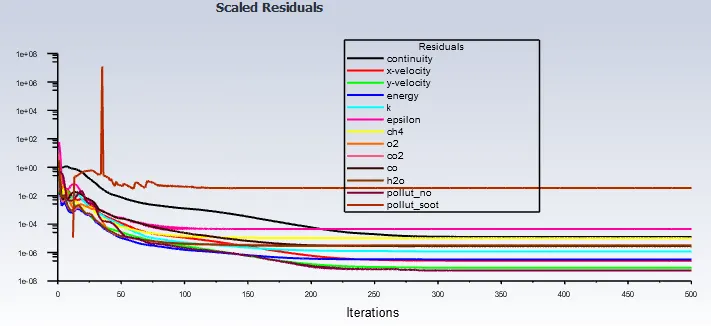
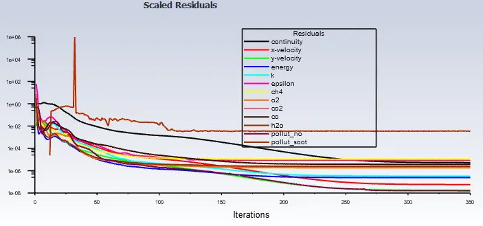
The simulation was run for 500 to 1000 iteration for each case and based on the simulation, the following results were extracted for each case.
Case 1
- Residual
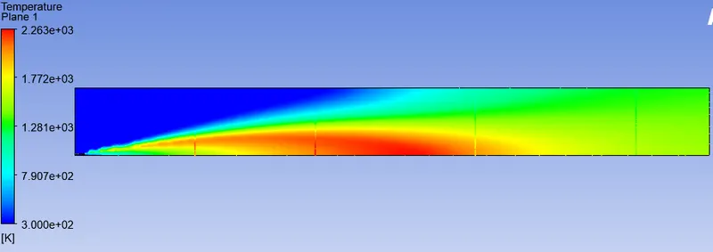
- Temperature contour
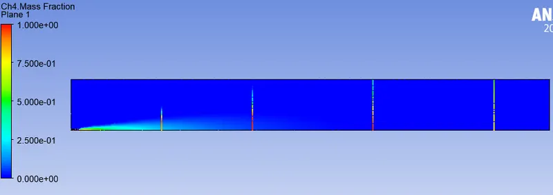
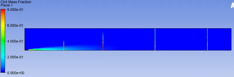
- Mass fraction of CH4
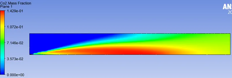
- Mass fraction of CO2
- Mass fraction of CO
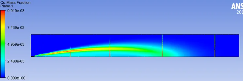
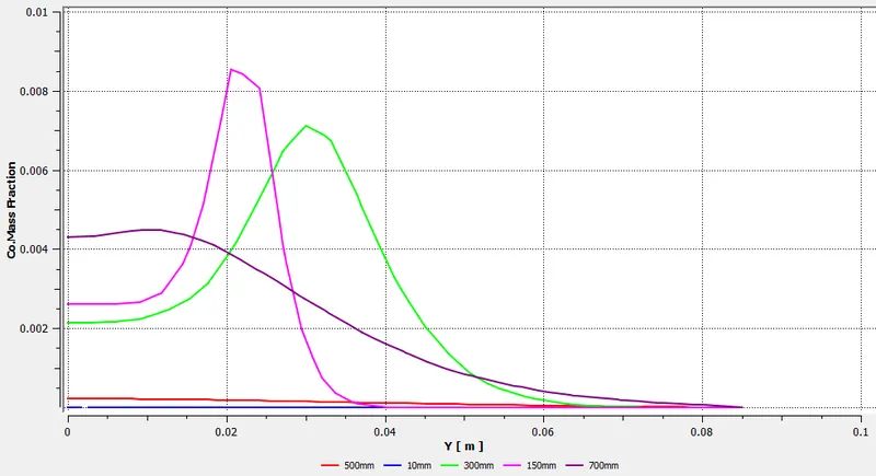
- Mass fraction of H2O
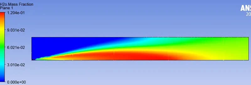
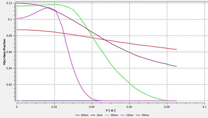
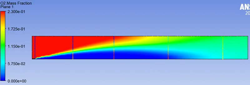
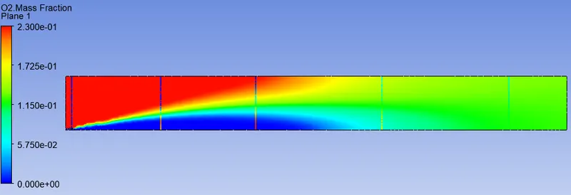
- Mass fraction of O2
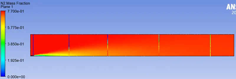
- Mass fraction of N2
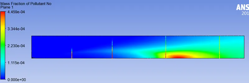
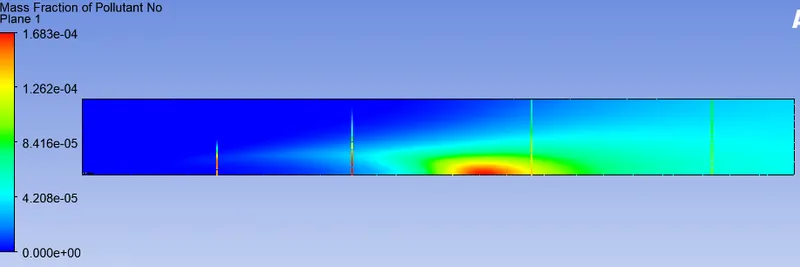
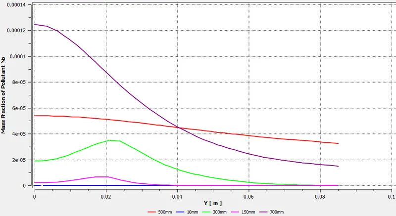
- Mass fraction of NOx
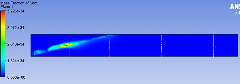
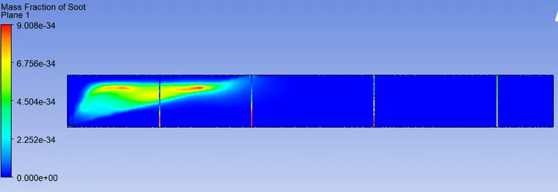
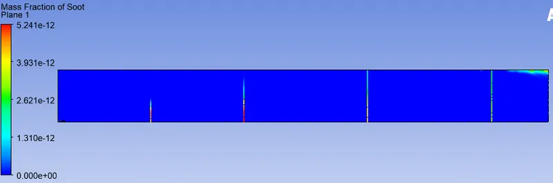
- Mass fraction of Soot
Case 2a
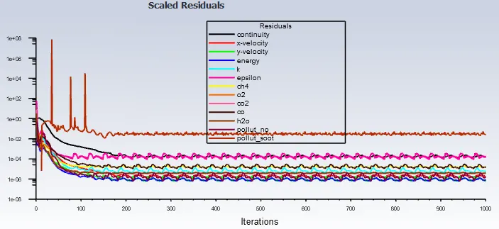
- Residual
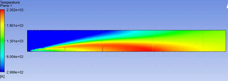
- Temperature contour
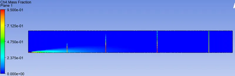
- Mass fraction of CH4
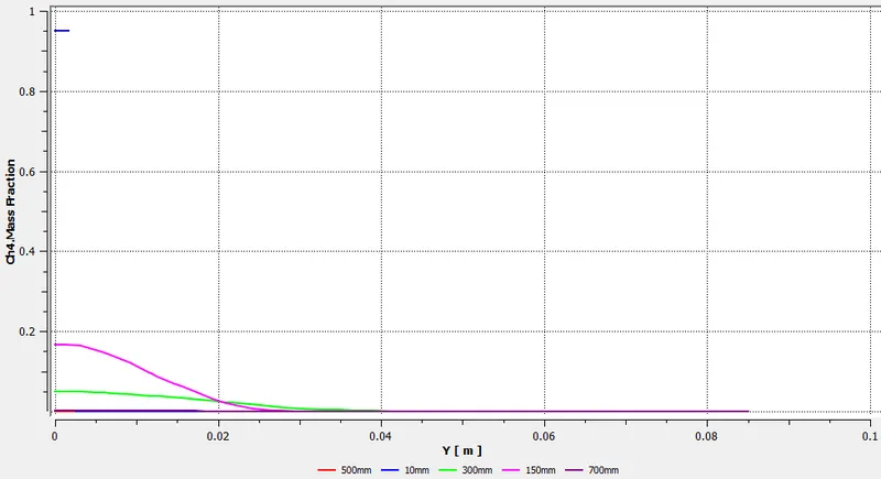
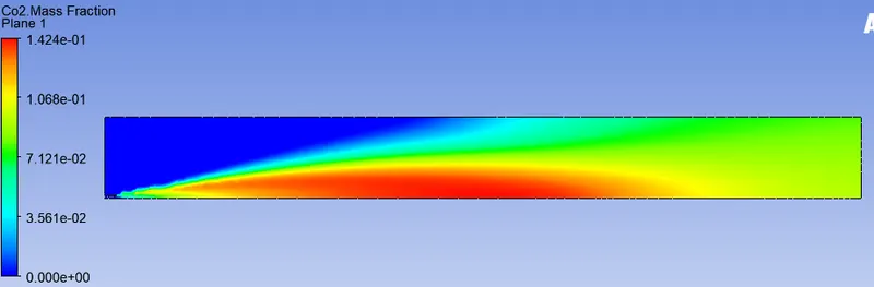
- Mass fraction of CO2
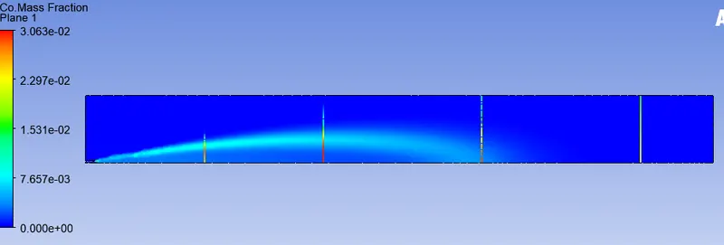
- Mass fraction of CO
- Mass fraction of H2O
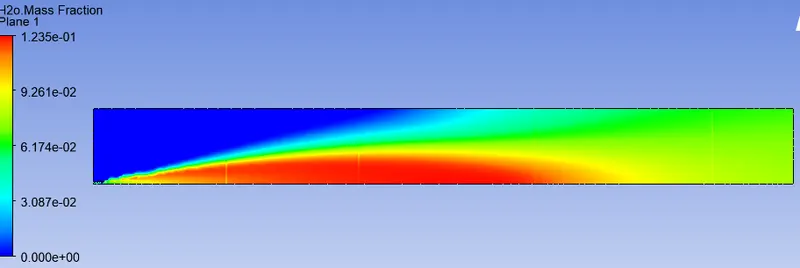
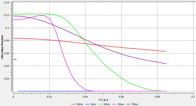
- Mass fraction of O2
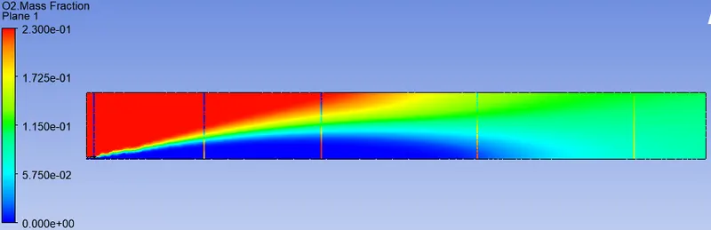
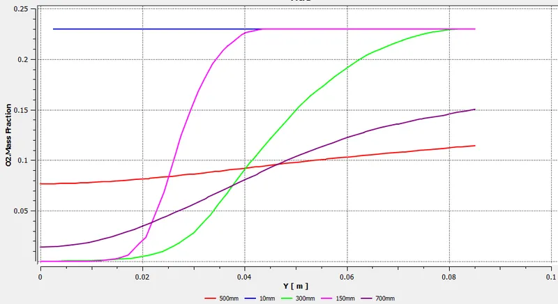
- Mass fraction of N2
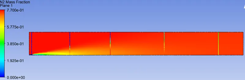
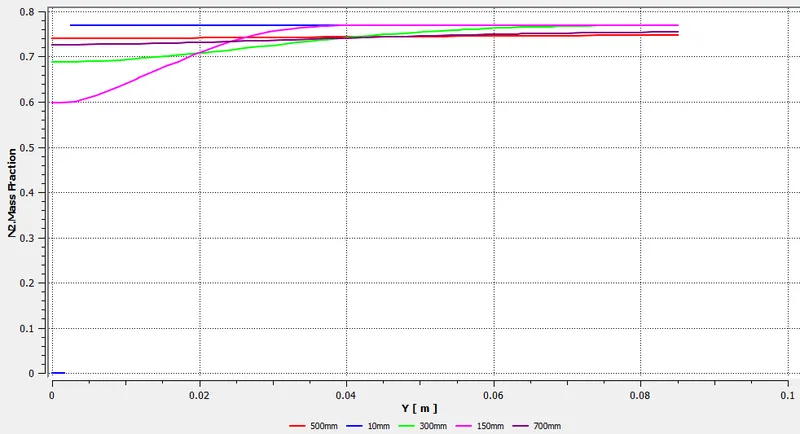
- Mass fraction of NOx
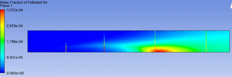
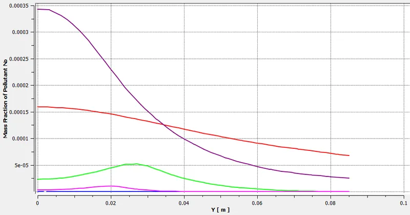
- Mass fraction of Soot
Case 2b
- Residual
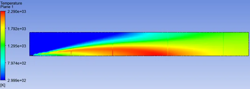
- Temperature contour
- Mass fraction of CH4
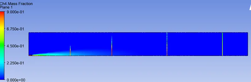
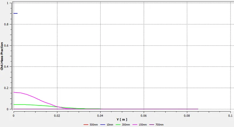
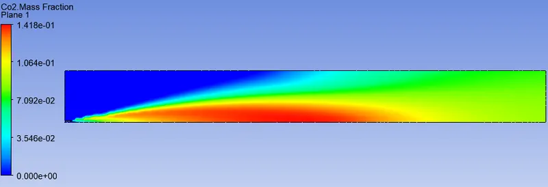
- Mass fraction of CO2
- Mass fraction of CO
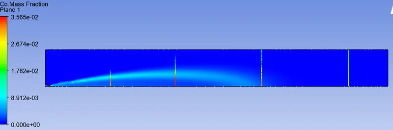
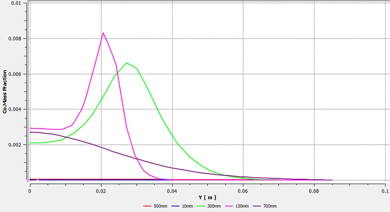
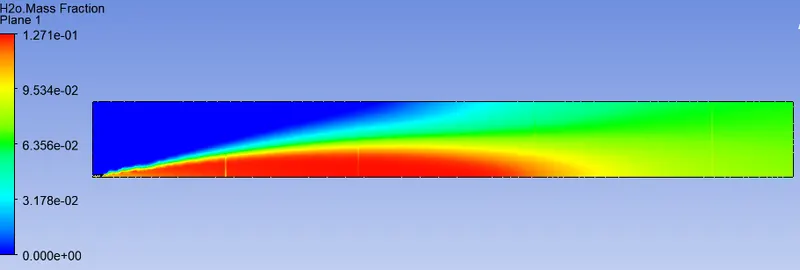
- Mass fraction of H2O
- Mass fraction of O2
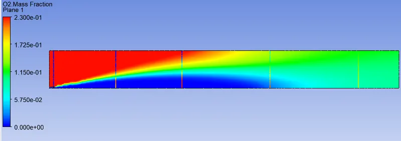
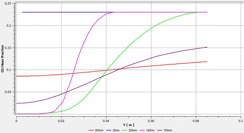
- Mass fraction of N2
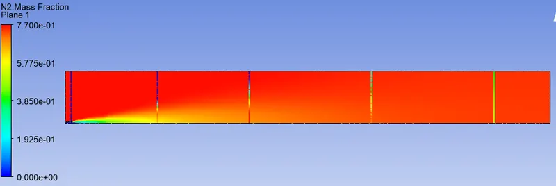
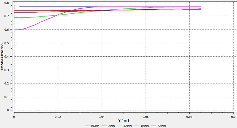
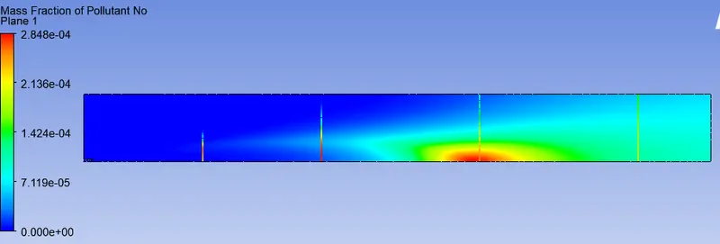
- Mass fraction of NOx
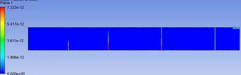
- Mass fraction of Soot
Case 2c
- Residual
- Temperature contour
- Mass fraction of CH4
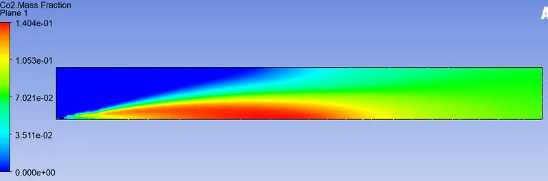
- Mass fraction of CO2
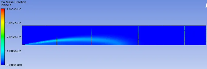
- Mass fraction of CO
- Mass fraction of H2O
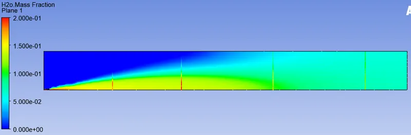
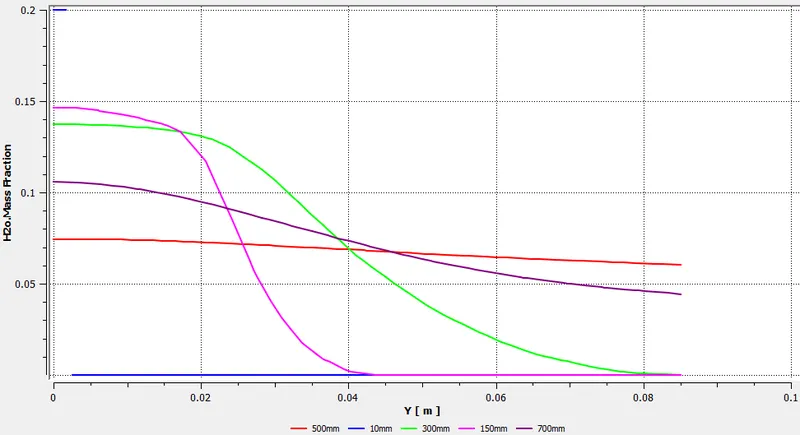
- Mass fraction of O2
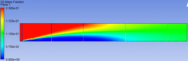
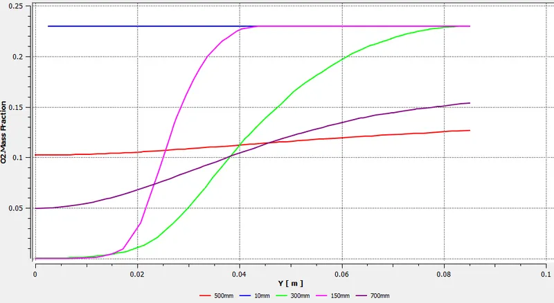
- Mass fraction of N2
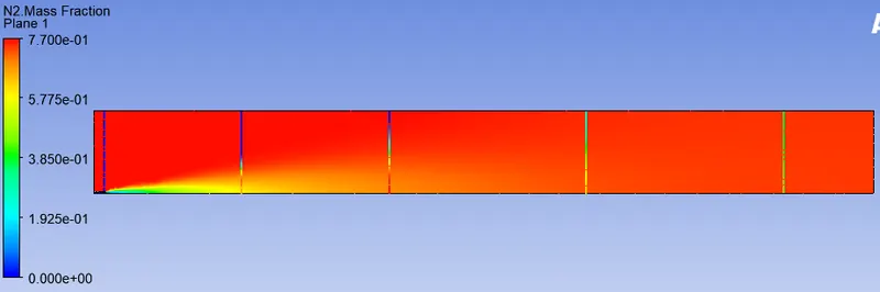
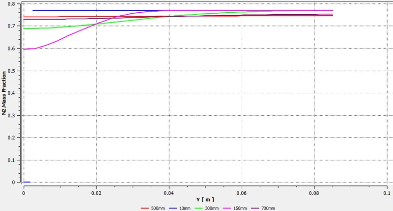
- Mass fraction of NOx
- Mass fraction of Soot
Case 2d
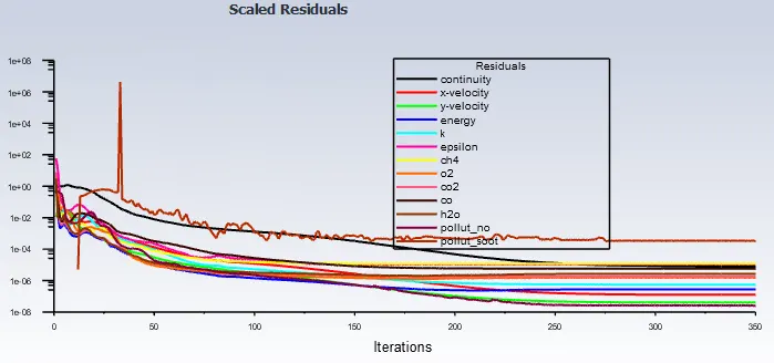
- Residual
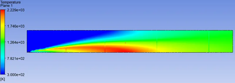
- Temperature contour
- Mass fraction of CH4
- Mass fraction of CO2
- Mass fraction of CO
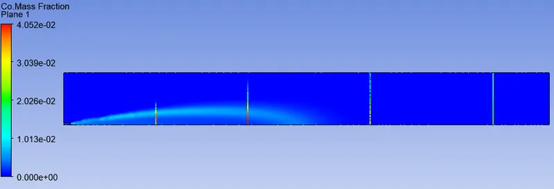
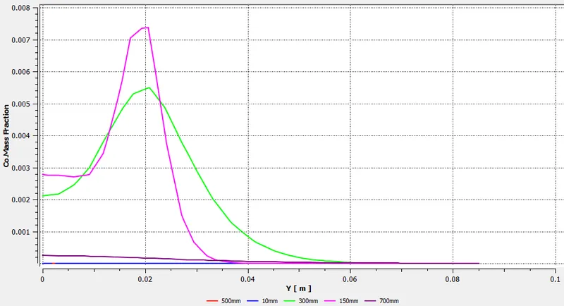
- Mass fraction of H2O
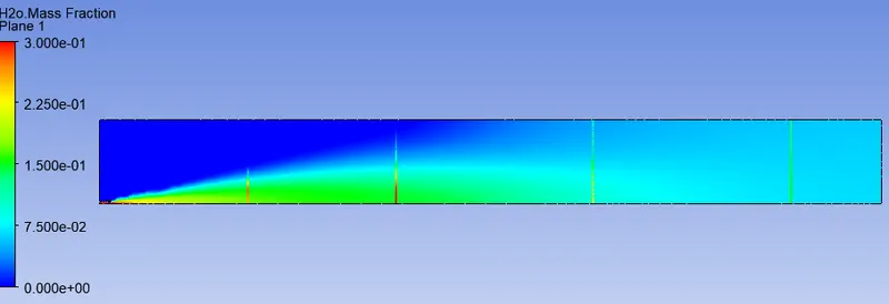
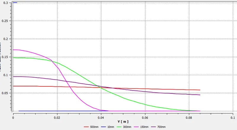
- Mass fraction of O2
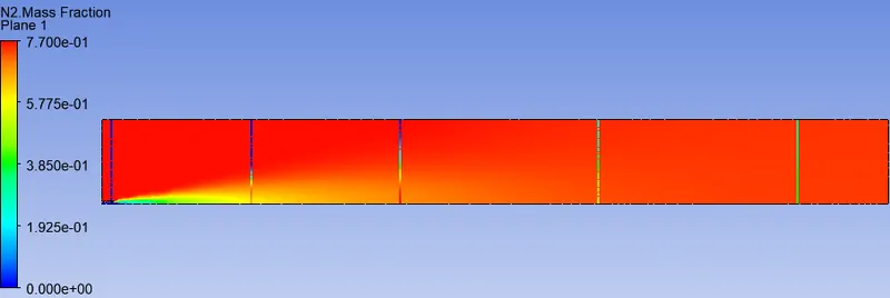
- Mass fraction of N2
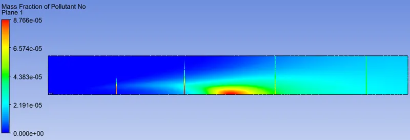
- Mass fraction of NOx
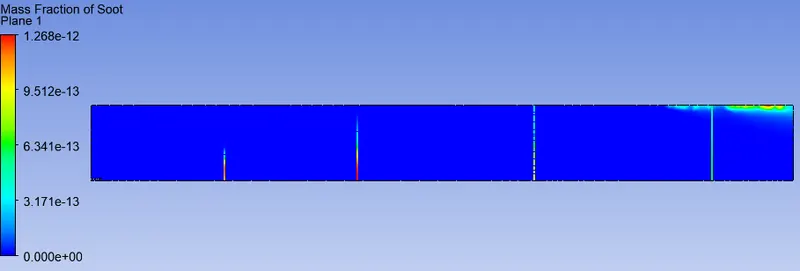
- Mass fraction of Soot
The below table shows the cumulative max values of mass fraction for each species in all the above-discussed cases.
| Temperature | CH4 | CO2 | CO | H2O | O2 | N2 | NOx | Soot | |
| Case 1 | 2312 | 1 | 1.429e-1 | 9.919e-3 | 1.204e-1 | 2.3e-1 | 7.7e-1 | 4.459e-4 | 5.296e-34 |
| Case 2a | 2302 | 0.95 | 1.424e-1 | 3.063e-2 | 1.235e-1 | 2.3e-1 | 7.7e-1 | 3.572e-4 | 9.008e-34 |
| Case 2b | 2290 | 0.9 | 1.418e-1 | 3.565e-2 | 1.271e-1 | 2.3e-1 | 7.7e-1 | 2.484e-4 | 7.222e-12 |
| Case 2c | 2263 | 0.8 | 1.404e-1 | 4.023e-2 | 2e-1 | 2.3e-1 | 7.7e-1 | 1.683e-4 | 5.24e-12 |
| Case 2d | 2229 | 0.7 | 1.386e-1 | 4.052e-2 | 3e-1 | 2.3e-1 | 7.7e-1 | 8.766e-5 | 1.26e-12 |
CONCLUSION
Based on the results discussed in the previous section, the table was prepared and the following inferences can be made
- With the addition of water the maximum temperature drops.
- The mass fraction of CO2 decreases whereas CO increases with the addition of water in the fuel.
- N2 remains almost constant for all configurations showing that it is almost inert throughout the reaction barring minute formation of NOx.
- An increase in water fraction in fuel results in a decrease in the formation of NOx. Also, the hotspot for max NOx comes nearer to the injector as the water fraction increases which can be confirmed from the Mass fraction contours of NOx.
- Soot formation increases as the water fraction increases in the fuel. Although the mass fraction is very low, the percentage change from 100 % fuel to 90% fuel+10% water is very large which shows that if the water is more in the fuel the formation of soot takes place and thus may result in a clog.
Note: The above study is conducted using eddy dissipation model which means the combustion ignition time is calculated based on the value of K and epsilon for the simulation. So even though, the results were fast, accuracy maybe questionable. In order to get the precise and accurate solution to combustion problem, Finite rate chemistry can be used which uses ODEs and reaction rate to determine the ignition time.