Bird Strike - Project - 2

Skill-lync project 2

Aim: The objective of this project is to set up an accurate model of a bird strike that simulates the impact of a bird on the blades of an aircraft jet engine. The simulation should be free of bugs and should show blade failure within a reasonable amount of time.

Case setup: The first keyword file contains a MAT24 material card, presumably defined as aluminium for the engine blades.

The second file contains the FE mesh for the engine and the bird, as illustrated below.

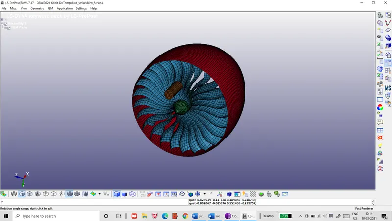Figure 1: FE mesh of engine and bird

It has default IDs for the elements, nodes and parts that are to be replaced so that node IDs start from 100000, element IDs start from 500000, part IDs start from 1000, and all other keyword IDs are within the 10000-19999 range. The different parts and control cards are to be stored as separate keyword files with a main file referencing these separate files for the simulation. The final simulation is to be prepared and debugged appropriately and the results compiled & verified.

Procedure: The files and simulation are prepared through the following sequence of steps.

1. The keyword file for the engine is imported into the LS-PrePost workspace. The blade part is then isolated while the remaining parts are removed.
2. The nodes, elements and parts have their IDs reset with the help of the renumber tool so that part IDs start from 1000, element IDs start from 500000 and node IDs start from 100000 respectively. Self-contact with a static friction coefficient of 0.12 and a dynamic friction coefficient of 0.1 is defined by the CONTACT>AUTOMATIC_SINGLE_SURFACE keyword with contact ID of 40000.
3. Steps 1 & 2 are repeated for the casing, hub and bird parts of the original keyword file. For each file, the element and node IDs are incremented by 50000.
4. The keyword file with the aluminium material card has the material ID for aluminium changed to 20000. An additional MAT077 (ogden rubber) material card is created for the bird with the following properties.
   1. Density: 1 X 10^-3 kg/mm³
   2. Poisson’s ratio: 0.499
   3. First shear modulus: 0.62 GPa
   4. First exponent: 1.3
   5. Second shear modulus: 0.00118 GPa
   6. Second exponent: 5
   7. Third shear modulus: -0.00981 GPa
   8. Second exponent: -2
5. A new keyword file is created with sections defined for the various parts. Section IDs start from 30000. Shell section with ELFORM=16 (fully integrated shell elements) is assigned to the shell elements. Solid elements are assigned solid section with ELFORM=4 (quadratic tetrahedron element with nodal rotations).
6. Another keyword file is created with control key cards for the simulation. The run time is set as 10 ms and the time step is set as 0.01 ms. Hourglass control and hourglass output are also set for the simulation.
7. In another keyword file, the output parameters are assigned via the DATABASE key cards. Here, the time step in the output files is set to 0.1 ms.
8. In a final keyword file, the files created earlier are imported via the INCLUDE keywords.
9. The different parts are assigned their respective section and material properties.
10. Contact between blades and casing, as well as between blades and bird is defined with the CONTACT>AUTOMATIC_SURFACE_TO_SURFACE keyword with a static friction coefficient of 0.12 and a dynamic friction coefficient of 0.1. A tied contact is also defined between the hub and the blades with the CONTACT>TIED_NODES_TO_SURFACE keyword.
11. A section at the top of the casing is constrained in all directions to simulate the engine mounting bracket. A CNRB is defined at the rear end of the hub, as shown below.

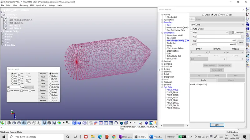Figure 2: CNRB at hub base

The master node of this CNRB is constrained in all directions except in rotational direction about the x axis.

12. The bird is assigned an initial velocity of 10 mm/ms. The hub and blades are assigned an initial rotational velocity of 0.5 rad/ms.
13. The model is then checked for errors, saved and run with LS-Run.
14. The resultant output files are then analysed using LS-PrePost. The first results that are analysed are the energy histories, both of the entire system and the individual parts.
15. The effective stress and plastic strain histories are plotted for an element in one of the blades.
16. The time step history is also checked for discrepancies.
17. Contact energies between the various contacts are compared.

Result: The following observations were made for the simulation.

• The animation shows heavy distortion in the blades with some of them breaking partially off the hub.
• The total energy plot shows that the total energy in the system is constant and the hourglass energy is negligibly small, as shown below.

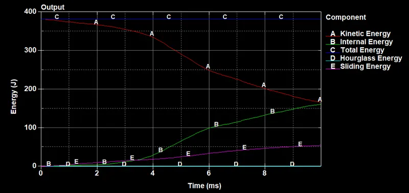Figure 3: Energy plot for entire system

This validates the accuracy of the simulation. The sliding energy is shown to be steadily increasing, which is representative of the various parts sliding against each other and themselves. The energies within the individual components are shown below.

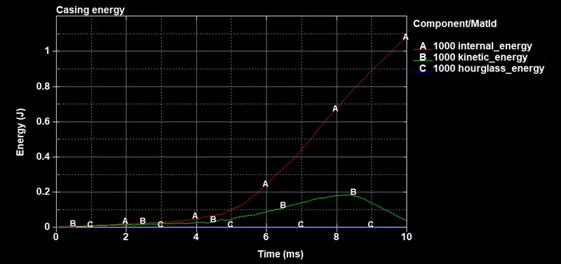Figure 4: Energy history of casing

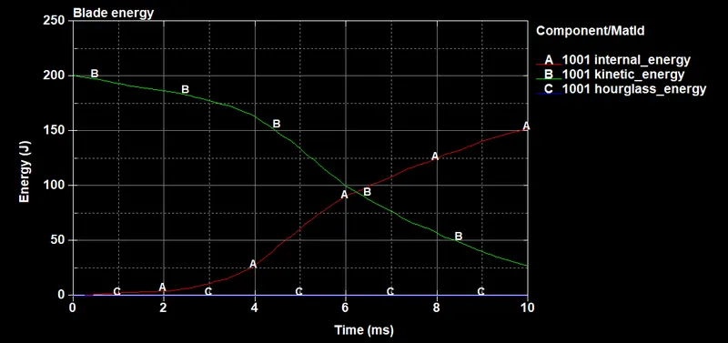Figure 5: Energy history of blades

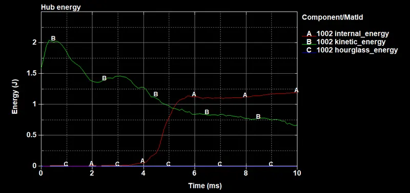Figure 6: Energy history of hub

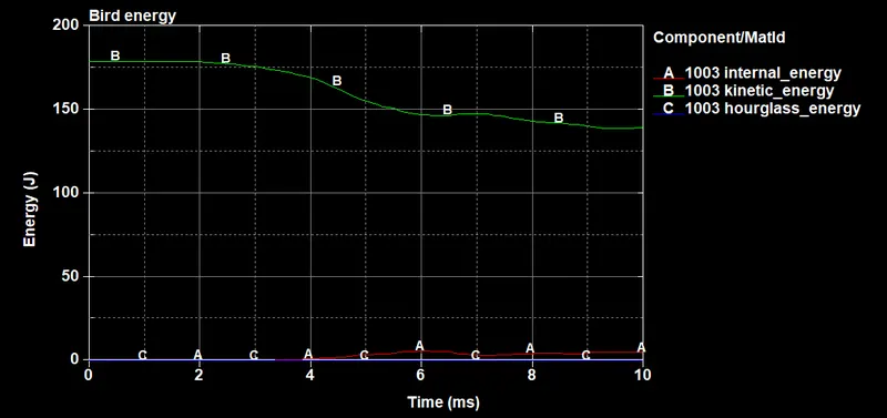Figure 7: Energy history of bird

They show that energy is ultimately lost from the moving components. The casing gains a small amount of internal energy, presumably from deformed blades rubbing against it. The bird loses kinetic energy with very little gain in internal energy, which shows that much of this kinetic energy is transferred to the blades. The blades show that decrease in kinetic energy corelates directly to an increase in internal energy. However, there is still a net loss of about 25 J of energy. This loss can be attributed to sliding energy loss between blades as well as the casing, and blade failure.

• The Von Mises stress and the plastic strain for an element on one of the blades at the point of impact are illustrated below.

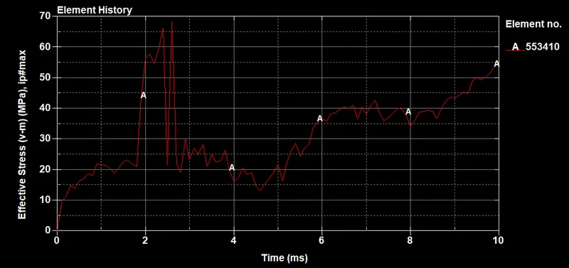Figure 8: Von Mises stress at point of impact

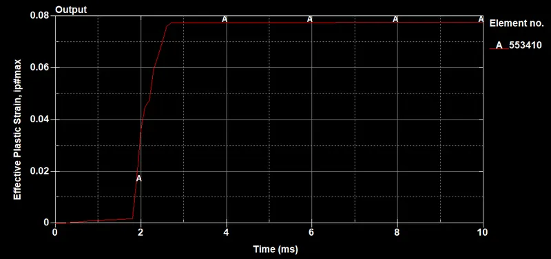Figure 9: Plastic strain at point of impact

They show massive spikes at the moment of impact, thus validating the accuracy of the simulation. The stress history shows that the spike is followed by a fall and a gradual rise. This rise could be from the neighbouring blades that press against the element as they deform.

• The time step history is illustrated below.

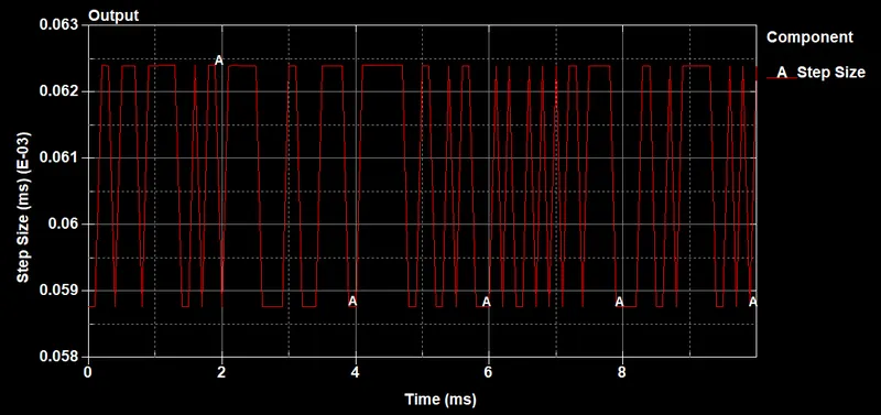Figure 10: Time step history

It shows a regular variation in the time step with no abrupt change in the pattern or deviation from the limits.

• The contact energies for all the contact defined are illustrated below.

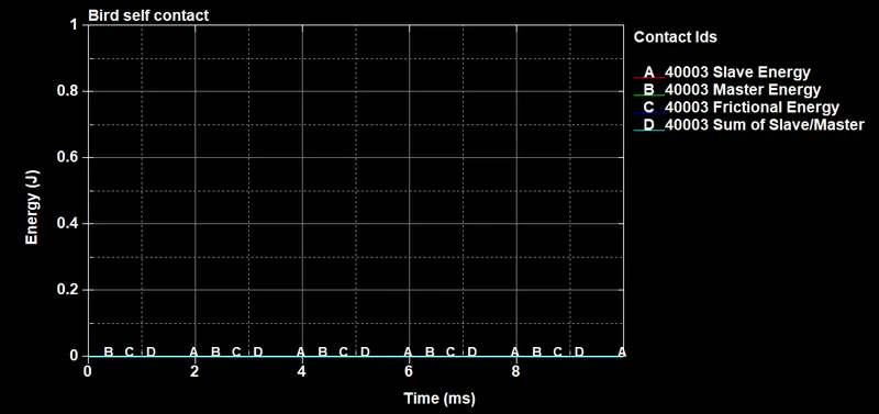Figure 11: Contact energies within bird

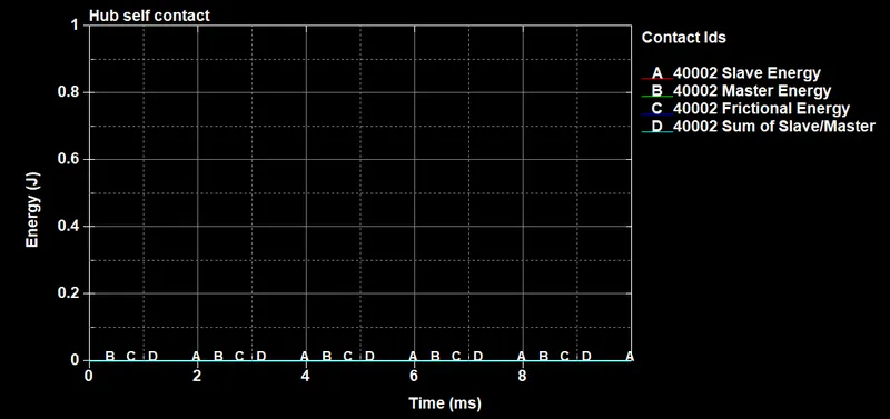Figure 12: Contact energies within hub

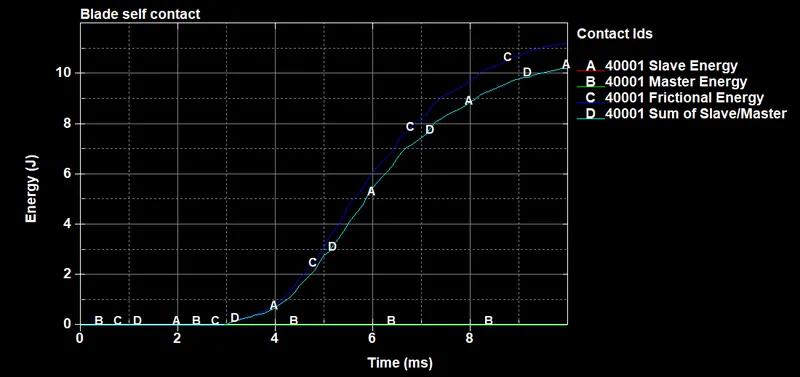Figure 13: Contact energies within blades

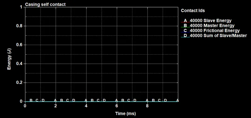Figure 14: Contact energies within casing

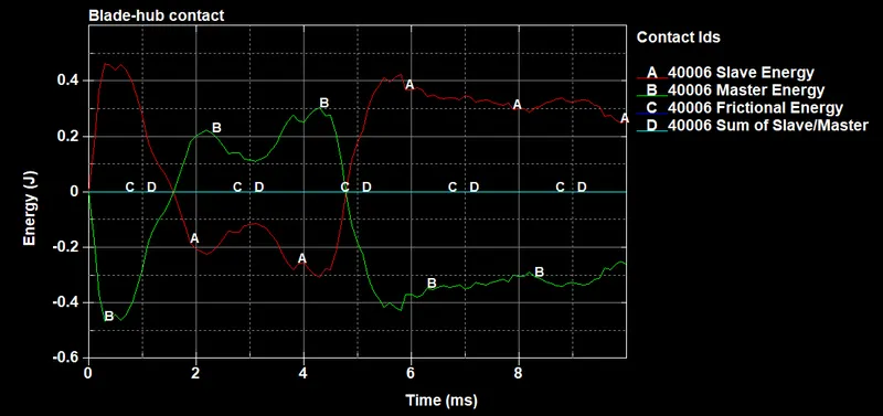Figure 15: Contact energies between blades and hub

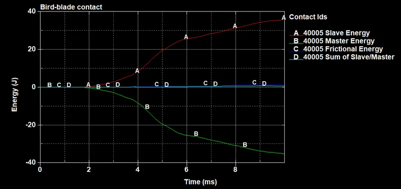Figure 16: Contact energies between bird and blades

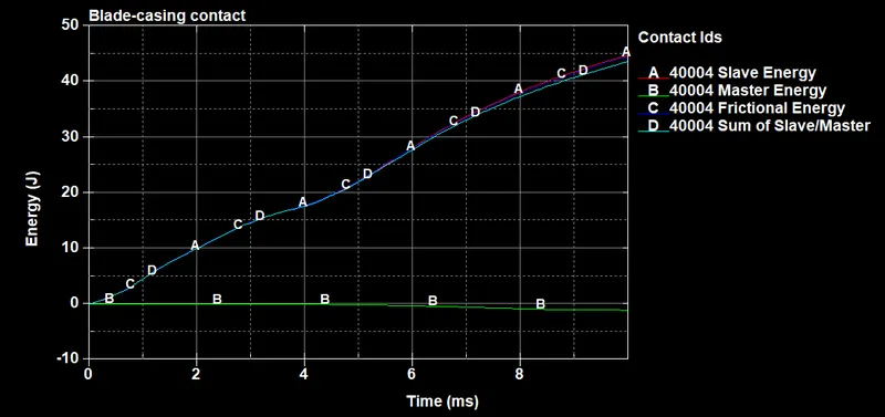Figure 17: Contact energies between blades and casing

The blades are the only parts that gain contact energies, which shows that only the blades experience self-contact. The contact energies between parts have a net sum of zero, while the slave and master energies are mirror images of each other, signifying a near perfect energy transfer between the parts. The exception to this rule is the contact between the blades and the casing. Since the casing is relatively stiff and is constrained, it cannot absorb much energy.

Conclusion: The simulation of a bird strike with the given component files was successfully executed. While it was not an accurate replica of the actual process, the observed energies, stresses and overall behaviour were similar enough to be representative of the same.