Assignment 7

Skill-lync assignment 7

Aim: The objective of this assignment is to simulate the side crash of the given component and generate time history plots for forces, intrusions and velocities in various sections. The energies are to be analyzed and discrepancies in the same be used to notice differences.

Case setup: The given component is a partial section of a car chassis which is illustrated below.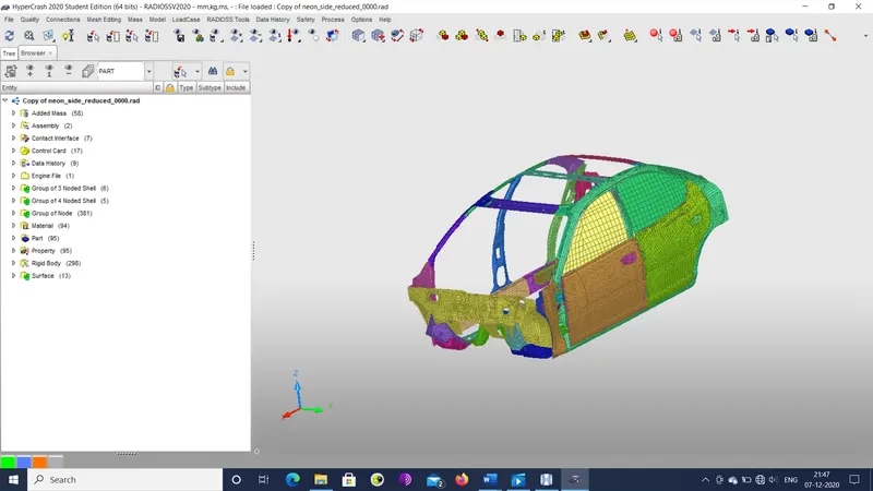

Figure 1: Component

The total mass of the component is 166.31 kg and the COG is located roughly at the driver side seat.

Procedure: The component is prepared for simulation and post-processed through the following set of steps.

1. The component is imported into the hyper-crash workspace and the units are checked for consistency.
2. The contact interfaces are replaced with a single type 7 contact with friction coefficient of 0.2, self-contact and other parameters optimized for accurate simulation.
3. The rigid bodies are modified so that center of gravity computation is set so that only slave nodes are considered.
4. The Federal Motor Vehicle Safety Standards (FMVSS) no. 201 is used as a basis for the initial velocity and rigid wall. The initial velocity is set by the load case>initial velocity menu selection. The value is set in the y direction and with a magnitude of 29 km/hr, i.e. 8.055555555 mm/msec.
5. A cylindrical rigid wall is added to the left side of the component by the load case>rigid wall menu selection. The wall diameter is set as 10 in or 254 mm. The wall friction is set as 0.1. The wall is then positioned until so that it is right next to the driver side of the car. The screenshot of the wall is shown below.

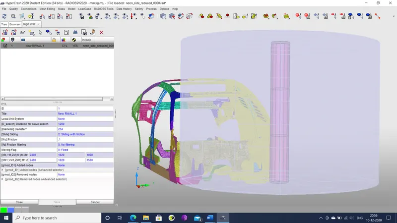
Figure 2: Pole definition (rigid wall)

6. The added masses are modified in order to bring the overall mass to 700 kg and shift the COG to between the front passenger seats. The masses are added to replicate the weights of a 120 kg front right door, a 120 kg, left side seat & driver combination, a 50 kg right side seat, a 150 kg rear seat and a 130 kg dashboard.
7. The model>control card menu selection is used to change animation parameters. In the DEF_SHELL section, the shell element formulation is changed to QEPH. In the DEF_SOLID section, the solid element formulation is changed to HEPH. In the DT_ELTYPE_KEYWORD_IFLAG section, the time step scale factor is set to 0.67, the time step control type is set to CST and the minimum time step is set to 0.1 microsec or 0.0001 msec for all element types. In the RUN section, the run time is verified to be 80 msec.
8. For the various cross-members, individual sections are defined where the cross-sectional forces are to be measured. The sections are added by the data history>section>section menu selection. One of these sections is illustrated below.

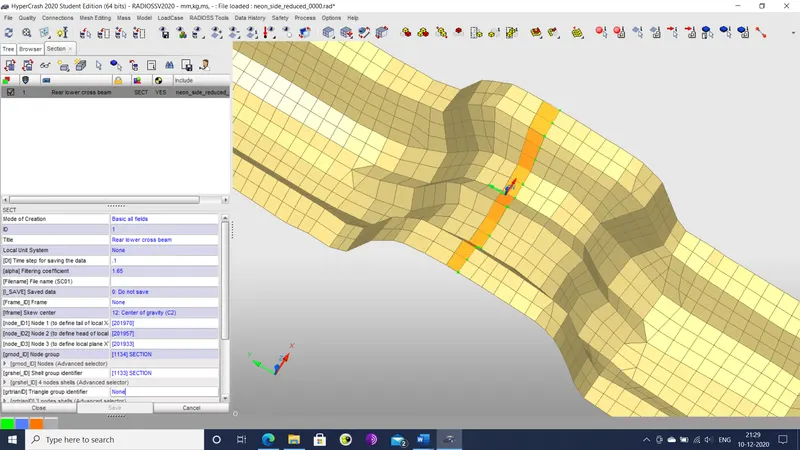
Figure 3: Cross section definition

9. For measuring the intrusions in the component, new type 13 springs are defined at the B-pillar, the front hinge pillar and the fuel tank. They are defined in a new part by the mesh editing>element>create menu selection. The springs are connected from said areas to the opposite end of the component that would presumably not deform during the simulation. The springs is also assigned almost negligible mass, inertia and stiffness. The springs are shown below.

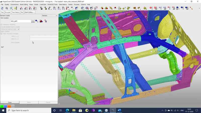
Figure 4: Virtual springs for intrusion measurement

10. For measuring velocities within the component, a skew is defined by the RADIOSS tools>skew/frame menu selection that acts a local frame of reference. Its location is shown below.

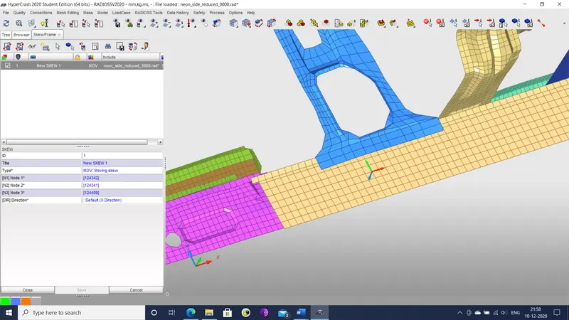
Figure 5: Skew definition

11. The data history>time history menu selection is used to bring up the time history plots that will be generated by the simulation. In the TH SECTION section, the variable being measured at the defined sections is changed to normal force (FN).
12. A TH SPRINGS section is defined for measuring the intrusion at the specified regions. The variable being measured is elongation in the y direction (LY).
13. A TH NODE section is defined for measuring the peak velocity of the inner side of the driver side door. The variable being measured is changed to velocity in the z-direction (VZ) with the local frame of reference being the earlier skew.
14. All the unnecessary time history plots are deleted from the model. The model is then checked for penetrations, after which the model checker is run to find any errors in the model and any found are rectified.
15. The output files are exported to a separate directory. The starter file from here is imported into the hyperworks workspace and the simulation is run in RADIOSS. The resultant animation files and time history plots are imported into the hyperview and the hypergraph 2D workspace respectively.

Results: The results from the simulation are examined and catalogued below.

• The overall simulation time was 2 hours 27 minutes and 58.17 seconds, while the number of cycles was 340814. The simulation time is due to the decision to keep the value of ICOG as 2, signifying that only slave nodes were used for COG calculation. Use of master slave only was dismissed as it was difficult to bring the COG to the necessary range under this parameter.
• The energy plot for the component is shown below.

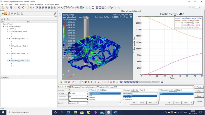
Figure 6: Energy plot

This plot is a near identical replica of the same in the previous assignment. The total energy is relatively constant, while there is a minor amount of contact energy being generated. This is the minimal amount of contact energy that can be generated, since the type 7 contact parameters are optimized as much as possible.

• The time step variation is shown below.

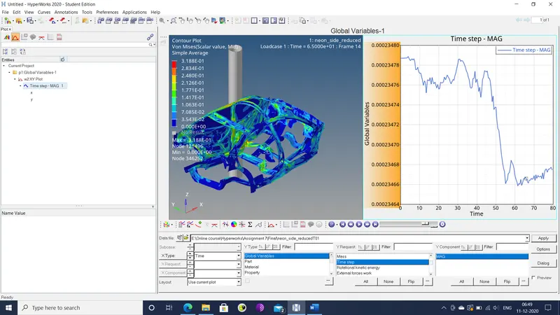
Figure 7: Time step plot

• It shows that it stays within the range of 0.1-0.5 microsec throughout the simulation. It is also apparent that at roughly the 55 msec mark, there is a minor drop in the time step until it levels out at a value 0.1 nanoseconds lower than the earlier. At first, this might indicate the activation of the time step correction algorithm. However, this is unlikely due to the low magnitude of the time step drop.
• The cross-sectional forces at the cross beams are plotted below.

Figure 8: Cross-sectional forces plot

• It shows that the lower cross beams are the first to fail. The peak value of force is 3.5 kg.mm/msec² or 3.5 KN.
• The plot of intrusions in the component is shown below.

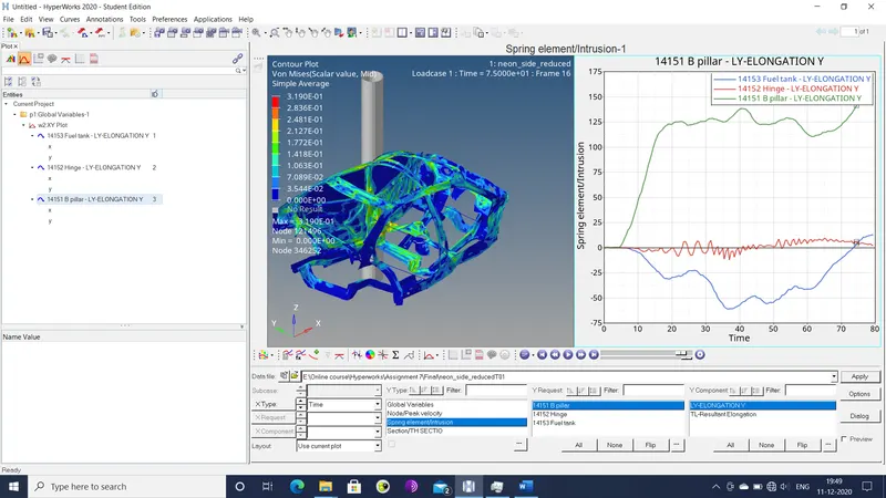
Figure 9: Intrusion plot

• It shows that the intrusion is the greatest at the B pillar, which is an accurate prediction. This intrusion reached 125 mm. The hinge pillar shows almost no intrusion. The fuel tank experiences an intrusion of 50 mm, after which it seems to drop. This is not accurate and this drop is due to the opposite end of the component also experiencing deformation during the later stages of the simulation, thus artificially reducing the intrusion.
• Judging by the location of the fuel tank, it can be inferred that the intrusion in the said area can be reduced either by thickening the sheet metal components of the tank/chassis or by shifting the tank further back in the chassis since the rear section deforms less than the middle of the component.
• The velocity of the inner side of the door is shown below.

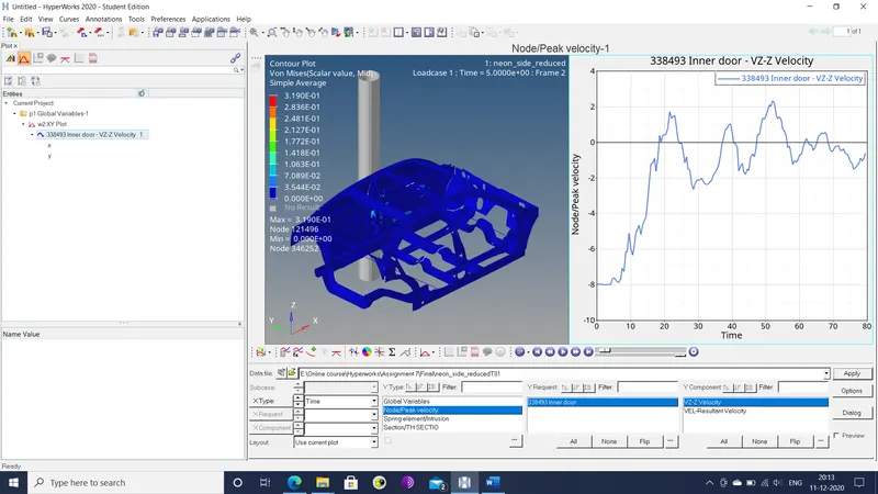
Figure 10: Velocity plot

• It shows that the actual velocity of the node rather than the velocity relative to the interior. It shows that the door decelerates from maximum speed of initial velocity to near zero. It does show significant fluctuation, which could signify an overtly high minimum gap activation for contact. This cannot be rectified easily since this value has already been set to a very low value of 0.5 mm.
• The 0001.out file verifies that time step does not drop significantly and the absence of mass change confirms that the time step scaling algorithm never activates in the simulation. The hourglass energy error reaches a minimum value of -1.5%.

Conclusion: The component was suitably preprocessed and simulated to observe the sectional forces, intrusions and velocities at the specified zones.