Assignment 6-Frontal Crash Simulation Challenge
Assignment 6-Frontal Crash Simulation Challenge
1. Aim
- Perform a frontal crash simulation with the mentioned model checks and procedures for the given model and find the answers for specified output requests.
2. Objective
Model Checks And Procedures for the Frontal crash-BIW
- Check the unit system and follow[Mg mm s] or [Kg mm ms].
- Create an appropriate interface, friction 0.2 and recommended parameters.
- Make sure of no penetrations and intersections.
- Correct rigid bodies if there are any issues.
- Create a rigid wall with friction of 0.1.
- Compare the model weight with the full-scale 300k nodes model and use added masses to reach a target weight of 700kg while getting CG about the required range.
- Initial velocity 35 mph.
- Use a model checker to ensure good quality.
- Time-step: 0.5 to 0.1 microseconds.
- Run 80 ms.
The Output Requests
- Sectional force in the rails at the location of indicated node 174247.
- The axial force received on the rails from the bumper.
- Shotgun cross-sectional forces.
- A pillar cross-section.
- Acceleration curve received on the accelerometer at base of B pillar (on B pillar rocker).
- Intrusions on the dash wall 66695,66244.
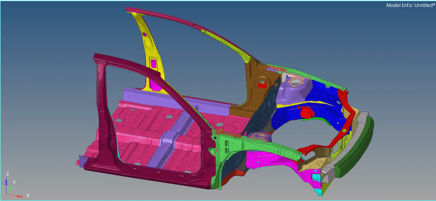
Fig 1: Isometric View Of Frontal Crash BIW Using Hyper Mesh
3. Procedure
Step 1: Importing of Model and Checking of Unit System
Initially import the model 'neon_front_0000.rad' to hypermesh using the solver deck. After importing we have to check the unit system specified on the model. It can be done by using a solver browser. From the solver browser, by clicking the 'Begin Card' we can see the unit system for the model. Because we have to use the same unit system for the entire crash test (for hyper-crash also). Otherwise, it will affect the results.
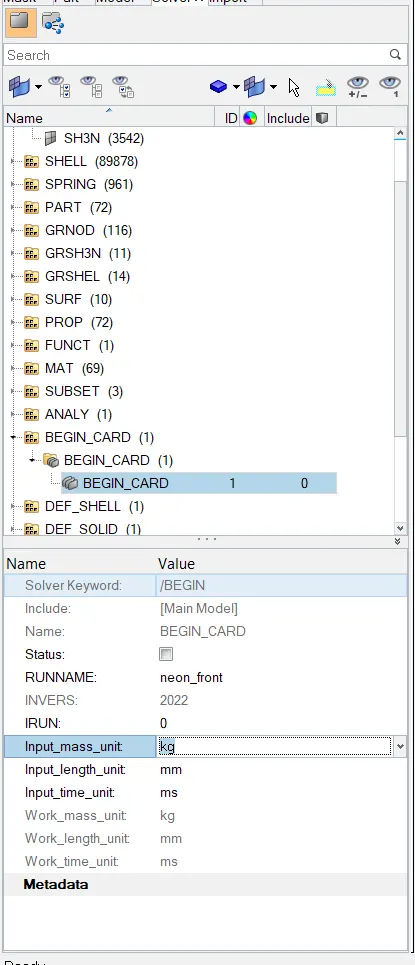
Fig 2: Checking of Unit System
So the unit system for the model is,
- Mass = Kg
- Length = mm
- Time = ms
Step 2: Penetration and Intersection Checking
Before the simulation, we have to make sure that there are no intersections (elements passing completely through one another) or penetrations (Overlapping of the material thickness of shell elements). The checking can be done by following,
- Tools (Menu Bar) >> Penetration Check >> Entity Type= Componets >> Selection= Select All Components >> Check.
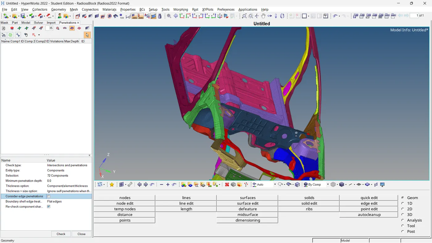
Fig 3: Penetration Checking Using Hypermesh
Step 03: Creating an Appropriate Interface With Recommended Values
A general node-to-surface contact or type 7 interface can be used for any application. The recommended parameters for type 7 include
| Sl No. | Parameter | Values |
| 1 | Istiff | 4 |
| 2 | Igap | 2 |
| 3 | Idel | 2 |
| 4 | Iform | 2 |
| 5 | Inacti | 6 |
| 6 | Stmin | 1 |
| 7 | GAPmin | 0.5 |
| 8 | Fric | 0.2 |
Table 1: Type 7 Parameters and Their Values
To assign a type 7 contact, go to the solver browser and right-click on,
- Create >> INTER >> TYPE7 >> Select Master and Slave >> Assign Recommended Values
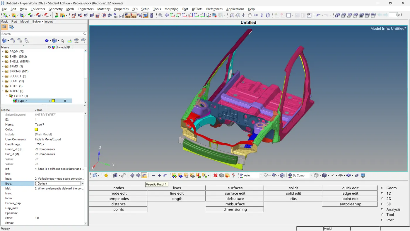
Fig 4: Assigning Interface Type 7
Step 4: Achieving Mass And CoG Of The Full-Scale Model.
Because it is one-third of the full-scale model (~30K Nodes), we have to achieve the same mass and CoG condition as this model.
- Tools (Menu Bar) >> Mass details >> Mass, Cog and Inertia >> Cog
The coordinates of the CoG point of a full-scale model is
Cogx = 3124.1047
Cogy = 5.7746
Cogz = 531.1952
For reference, created a node in the current model, using the CoG coordinates of the full-scale model.
and the CoG coordinates of the current model are,
Cogx = 3162.7577
Cogy = -2.7368
Cogz = 439.6496
From the question, we can see that the total mass = 700 Kg, and the mass of the current model is 188 Kg, We have to add an extra 512 Kg in the proper place to make the mass and location of CoG consistent. For that, we use hypercrash. Import the RADIOSS file to the hyper crash that was saved from hypermesh.
We have to isolate a part to add the additional mass. By analysing the coordinates of both models, the coordinates of the x-axis are nearly the same. Also, the gap between the z-axis is tiny. Only the y coordinates need some changes from their location. By considering these points, using the 'Isolate Selected Parts' option', select the component 'CH-RAILS-U-FT-CTR (ID=397)'. Then add mass to the nodes of these components by,
- LoadCase >> Added Masses >> Create New Object >> Select Type= 1(Mass is distributed to each node of the node group) Give Title >> Mass=512 >> Grnod_Id(Support)= Right Click >> Select In Graphics >> Add/Remove By Picking Selection >> Select Nodes >> Yes >> Save.
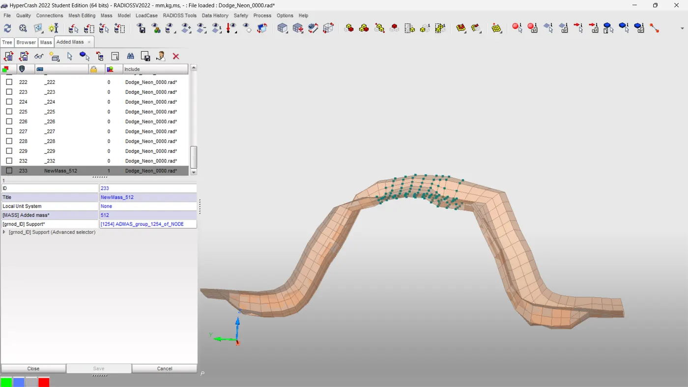
Fig 5: Adding Mass To The Model
Check the updated Cog coordinates by,
- Mass >> Balancing
The Cog coordinates are updated and the values of updated coordinates are,
Cogx = 3239.559
Cogy = 5.8074
Cogz = 403.6565
Step 5: Appling Initial Velocity To The Model
As per the objective, we need to define the velocity of 35 mph for the model. We have to convert the unit to mm/ms. That gives
35 mph = 15.65 mm/ms.
Using the hypercrash again, we can assign the velocity to the whole model. We need only the translational velocity in the x direction.
- LoadCase >> Initial Velocity >> Create New Object >> Give Title >> Select Type= 0: Translational>> Vx=15.65, Vy=0, Vz=0 >> Gnod_Id(Support)= Right Click >> Select In Graphics >> Include Picked Parts >> Select Whole Parts >> Yes >> Save.
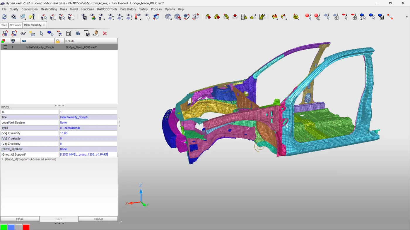
Fig 6: Assigning Initial Velocity
Step 6: Creating a Rigid Wall
A rigid wall is a nodal constraint applied to a set of secondary nodes to avoid node penetration to the wall. For creating the rigid wall, we can use hypermesh.
- Right Click On Solver Browser >> Create >> RWALL >> PLANE
After that, we have to assign proper values to RWALL. For the coordinates of the base node, we can define using a temp node. The normal should be along the '-x axis'. Other assigned values are
- Slide = 2: Sliding With Friction
- Dsearch = 1500
- FRIC =0.1
Assign the TH_Rwall file for the rigid wall. Make sure that, you select the required variables so that it improves the efficiency of the simulation
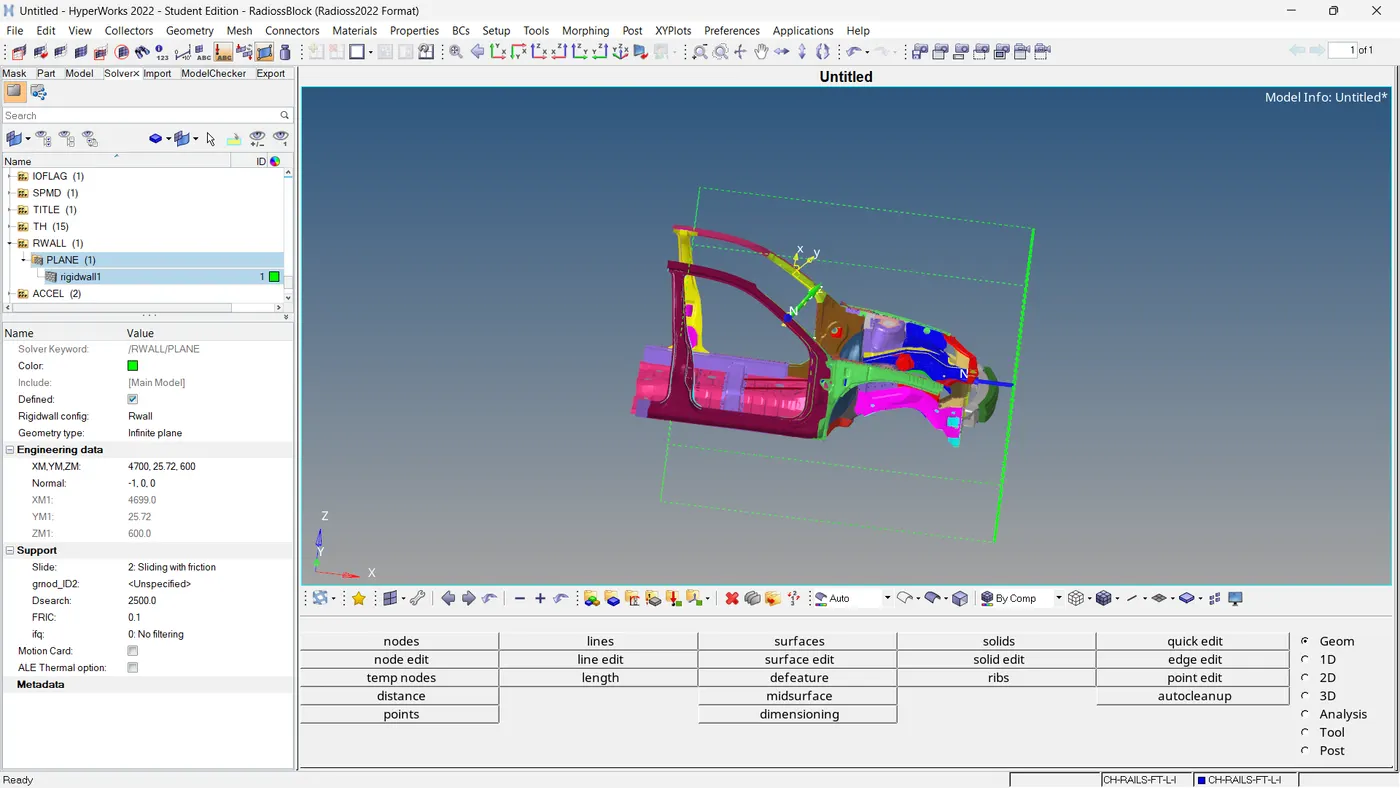
Fig 7: Creating RWALL
Step 7: Intrusions on the dash wall 66695,66244.
Here we have to find the displacement of these mentioned nodes in the dash wall. For that, we can define a spring as having very small stiffness. And we can find the displacement of those springs with the TH file. To create spring, go to the solver browser and right-click on,
- Create >> Elements >> Spring >> Spring2N >> Define one node by node ID and the other node in the cross member.
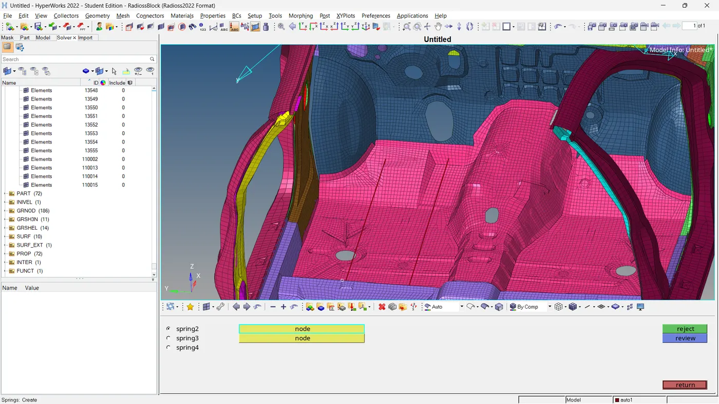
Fig 8: Spring Element Settings
Create a spring property card having the values of K=0.001 and M=0.001. Assign these properties to the newly created springs. Create separate TH_Spring files for these springs. Make sure that, you select the required variables so that it improves the efficiency of the simulation
Step 8: Accelerometers Setup
For the Acceleration curve received on the accelerometer, we have to implement an accelerometer at the base of the B pillar (on the B pillar rocker). We have to construct two of them one on each side. To create an accelerometer, go to the solver browser and right-click on,
- Create >> ACCEL >> Rename >> node_ID =Select the node where we need the accelerometer >> Proceed.
Assign separate TH_ACCEL files for these accelerometers. Make sure that, you select the required variables so that it improves the efficiency of the simulation
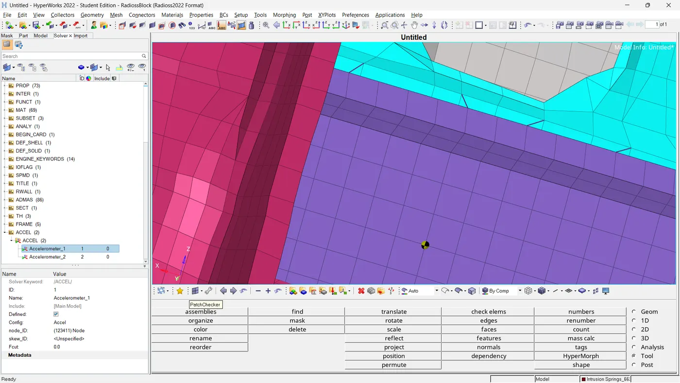
Fig 9: Accelerometer Setup
Step 9: Sections
As per the output requests, we have to create sections across both A-pillars, both shot-guns and node ID 174247. Before this, we have to make frames at these mentioned locations. These are used in sections as a Frame ID. For that, go to the solver browser and right-click on,
- Create >> FRAME >> MOV >> Select Origin Node >> Select Node To Define Axis >> Select Node To Define Plane.
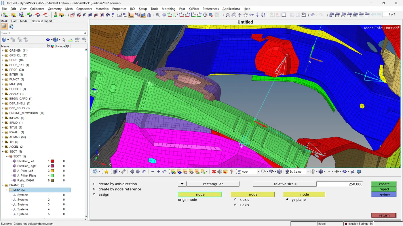
Fig 10: MOV Frames
The construct sections with these frames. From the solver browser,
- Create >> SECT >> SECT >> Select N1, N2, N3 for the Normal Direction>> Frame_ID =Select System corresponding MOV frames ID >> grShel_ID >> Right Click >> Select required nodes from part >> delta T=0.1.
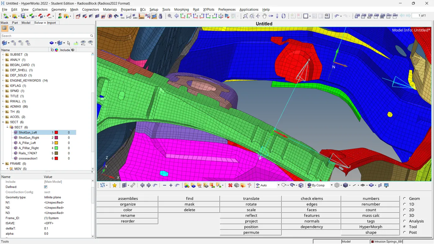
Fig 11: Sections
After making the required sections we have to assign a time history for every section. Make sure that, you select the required variables so that it improves the efficiency of the simulation
Step 10: Model Checking
Before the simulation, we have to make sure that, the model is error-free and ready to simulate. So initiate a model check by,
- Tools >> Model Checker >> RadiossBlock
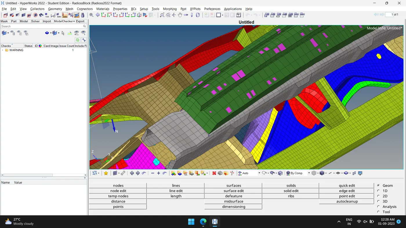
Fig 12: Model Checking
After the checking, there are some unused sets and other minute errors. The model checker automatically resolves those. Apart from a warning, the model has no other issues and is ready for the simulation. Check the minimum time step and total run time.
Step 11: Simulate the Model and Analysis of the Results
The simulation is done by following,
- Analysis >> Radioss >> Browse Input File Location >> Option = -nt 4 (No. Of Threads) >> Radioss
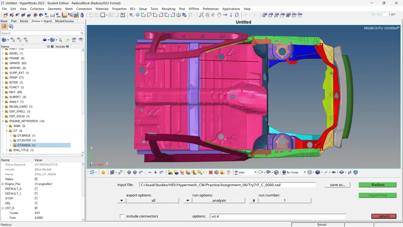
Fig 13: Loading Simulation Using Hyper Mesh
4. Observations And Conclusions
After the simulation, we have to check the job summary to analyse the results. It decides whether the results are acceptable or not.
From the output file,
- Energy Error = -2.5%
- Mass Error = 0.001177%
- Mass Addition = 0.8228
- Engine Run Time = 4314.75 s
- Total No. Of Cycles = 160001
The errors are within the acceptable range. So we can continue with the model.
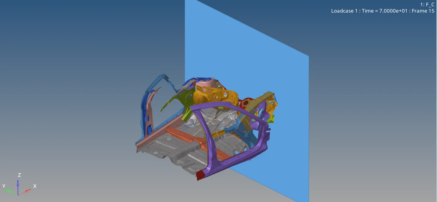
Fig 14: Animation Of Simulation
1. Von Mises Stresses
To get Von Mises Stress distribution, load the '.h3d file' in hypergraph and select the contour type as a Von Mises Stress.
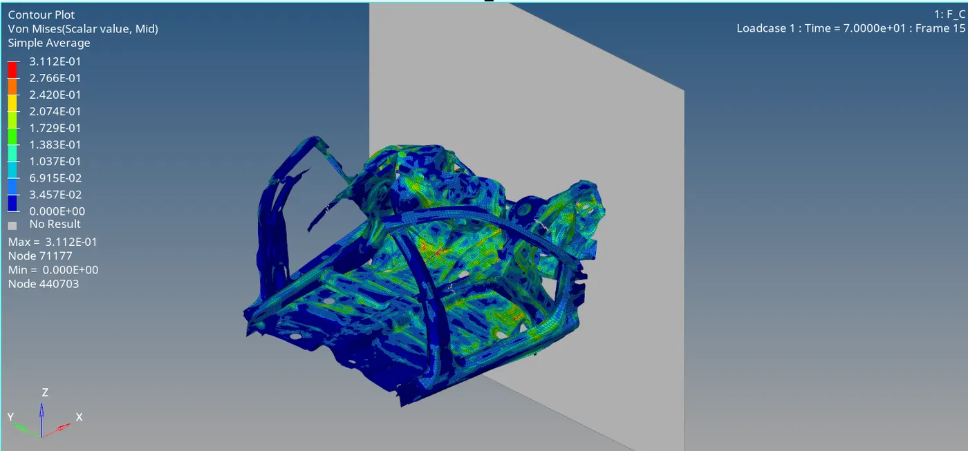
Fig 15: Von Mises Stress Distribution
By analysing the animation,
- Von Mises Stress (Max) = 3.112E-01 KN/mm2 at node 71177.
= 311.2 N/mm2
= 311.2 Mpa
From the simulation, initially, the bumper made contact with the rigid wall. So the number gets maximum deformation from the collision and then the forces are reduced throughout the simulation because of the energy absorption of each component.
2. Energy Graphs Of The Simulation
By loading the time history file (T01) to Hypergraph 2D, we can plot the necessary graphs and analyse the results.
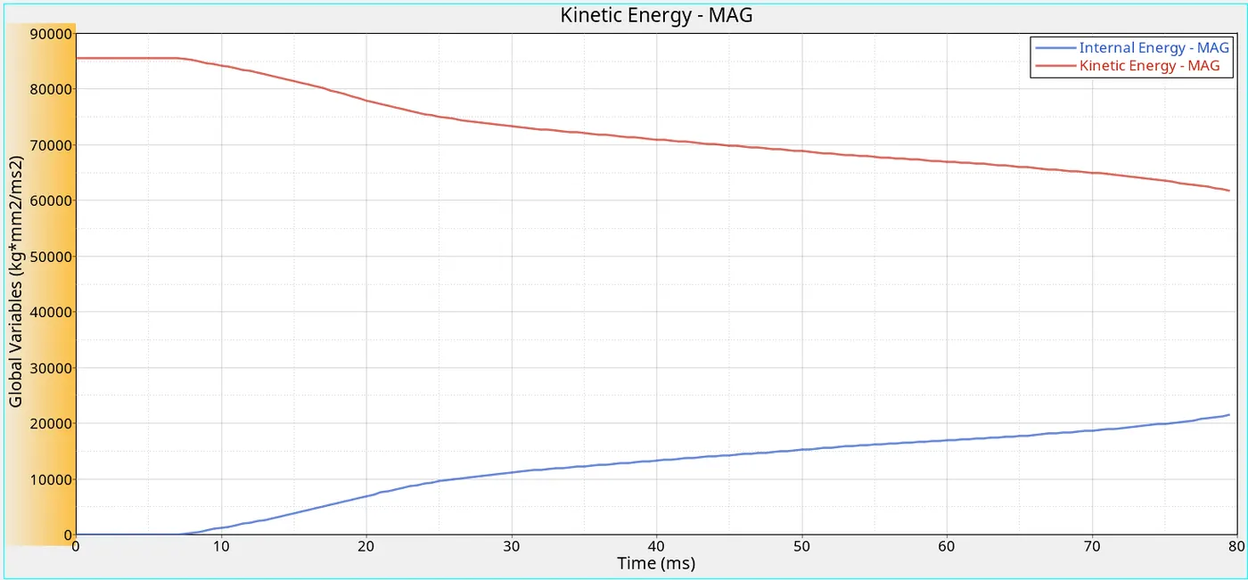
Plot 1: Time Vs Internal Energy / Kinetic Energy
From the plot, we can see that the collision did not happen for the first 6.5ms, so the kinetic energy is at peak value and the internal energy is at zero. After 6.5ms the collision with RWALL at 15.66 MpH speed, the kinetic energy starts decreasing but the internal energy starts to rise. The internal energy increases with the decrease of kinetic energy.
| Sl No | Time (ms) | Internal Energy (Kgmm2/ms2) (Joules) | Kinetic Energy (Kgmm2/ms2) (Joules) |
| 1 | 0 | 0.00 (Min) | 85591.28 (Max) |
| 2 | 6.5 | 6.817 | 85591.28 |
| 3 | 7 | 32.231 | 85545.25 |
| 4 | 30 | 11180.16 | 73321.06 |
| 5 | 79.5 | 21472.62 | 61746.46 |
Table 1: Time Vs Internal Energy / Kinetic Energy
Take account of the hourglass energy and total energy plots. The total energy is slightly reduced as the simulation runs, it is because of the presence of minute hourglass energy. Because of the Improved under-integrated element formulation method (QEPH), the majority of hourglass energy is controlled by physical stabilisation. So the hourglass energy is negligible compared to total energy.
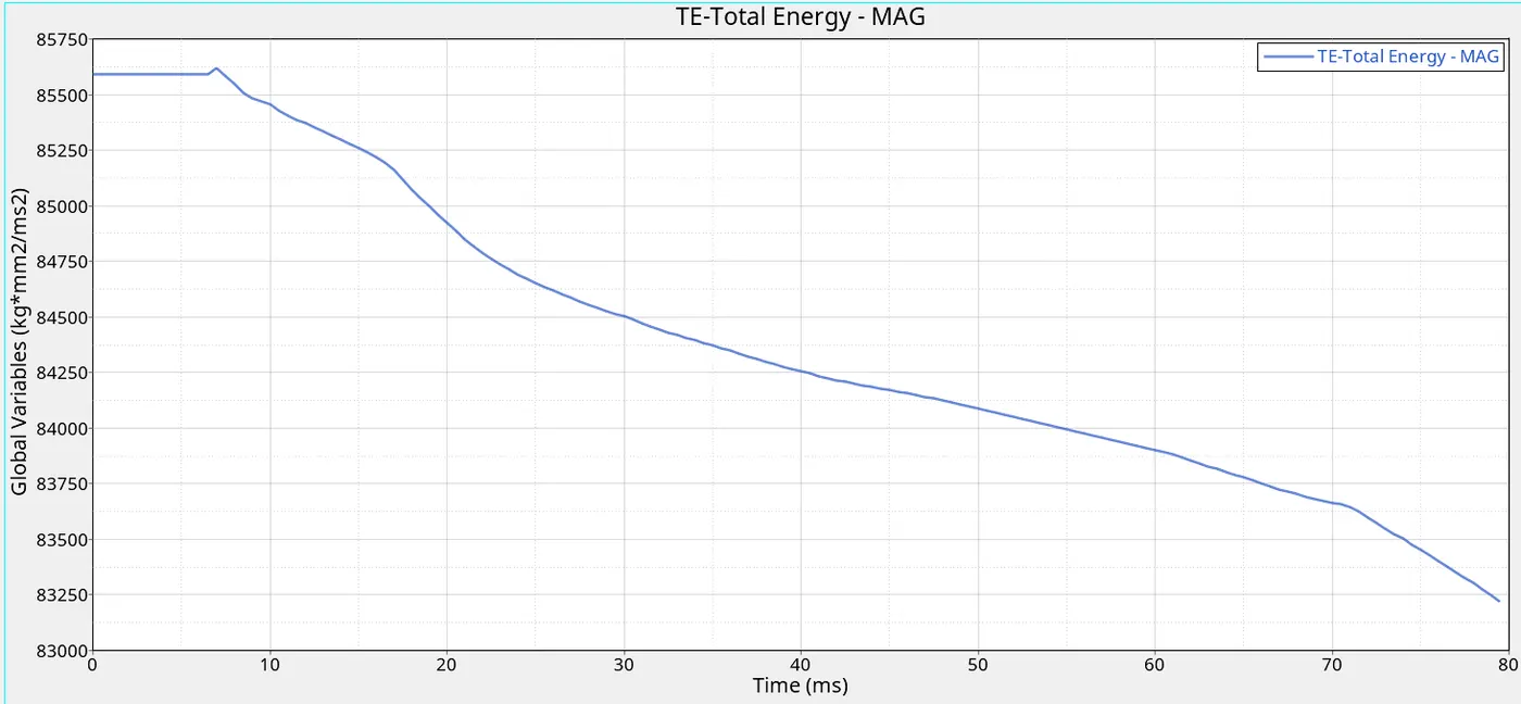
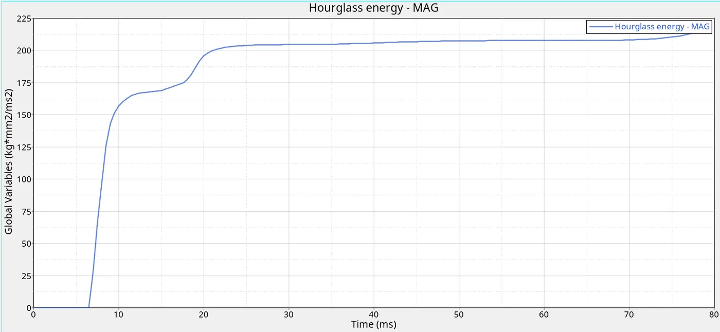
Plot 2: Time vs. Total Energy Plot 3: Time vs. Hourglass Energy
| Sl No | Time (ms) | Total Energy (Kgmm2/ms2) (Joules) | HourGlass Energy (Kgmm2/ms2) (Joules) |
| 1 | 0 | 85591.28 (Max) | 0.00 (Min) |
| 2 | 6.5 | 85591.27 | 7.6e-28 |
| 3 | 7 | 85620.28 | 28.256 |
| 4 | 10 | 85453.625 | 157.078 |
| 5 | 25 | 84652.25 | 203.931 |
| 6 | 79.5 | 83219.05 | 221.377 |
Table 2: Time vs. Total Energy / Hourglass Energy
3. Sectional force in the rails at the location of indicated node 174247
To find out the sectional force in the rails at the location of the indicated node, we have to plot the sectional forces on the location where node 174247 is located. By inspecting the results, the force started to be exerted almost at the beginning of the contact with the rigid wall. It's also because the search distance of the Rwall is high that it includes these sections at the beginning of the collision. The force is increasing rapidly for the first 10ms from the contact begins and reaches to its maximum value. Then gradually decreases to a certain value.
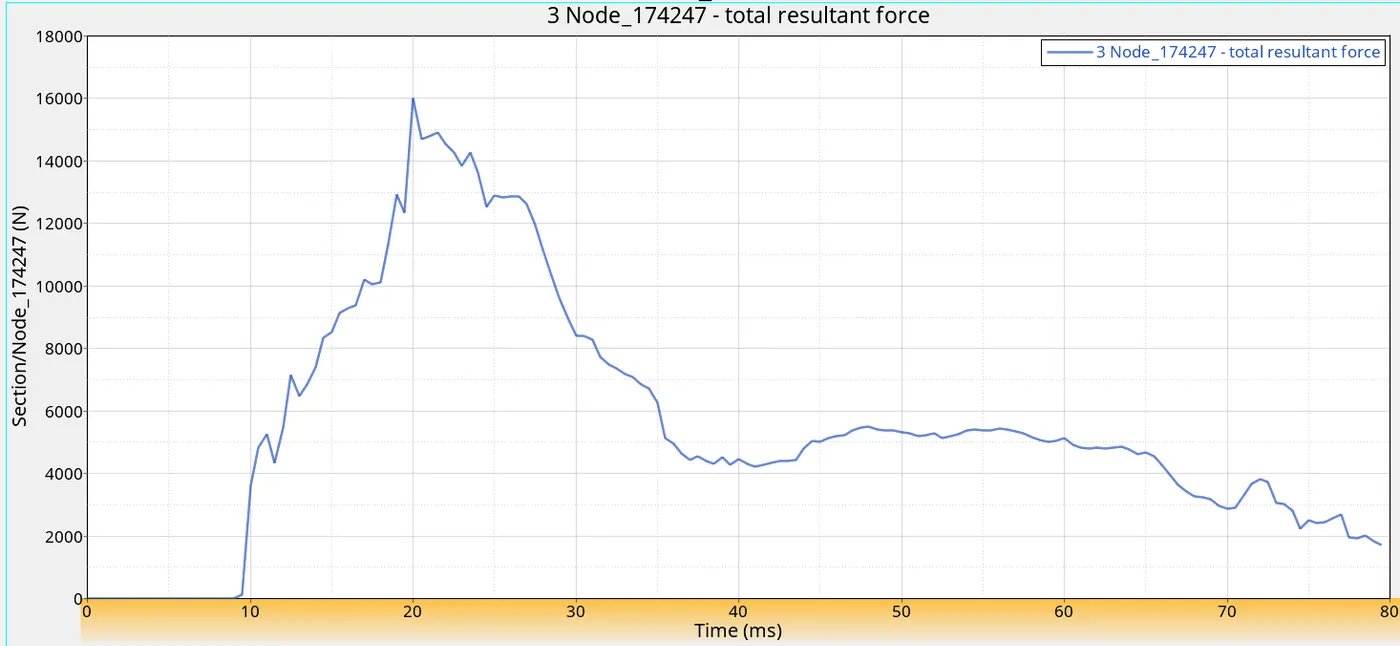
Plot 4: Time vs. Total Resultant Force (Node 174247)
| Sl No | Time (ms) | Total Resultant Forces (N) |
| 1 | 0 | 0.00 (Min) (~1.055e-15) |
| 2 | 9 | 0.9921 |
| 3 | 10 | 3600.533 |
| 4 | 20 | 16019.21 (Max) |
| 5 | 50 | 5321.667 |
| 6 | 79.5 | 1701.662 |
Table 4: Time vs. Total Resultant Force (Node 174247)
The max total resultant force experienced 17427= 16019.21 N
= 16.019 KN at t=20ms
4. Shotgun cross-sectional forces.
By following the same procedure as previously, we can plot and inspect the cross-sectional forces on the Shotgun situated on the both left and right sides of the vehicle. In SG_Right plot 5, the force is exerted just after the collision takes place. After that a sudden leap in the plot and a small decrease in force and then rises to its maximum value. Plot 6 for the SG_Left, follows almost the same nature. The only difference is here the total resultant force is higher in SG_Left than SG_Right.
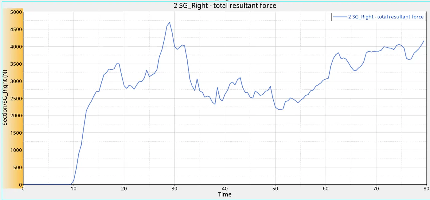
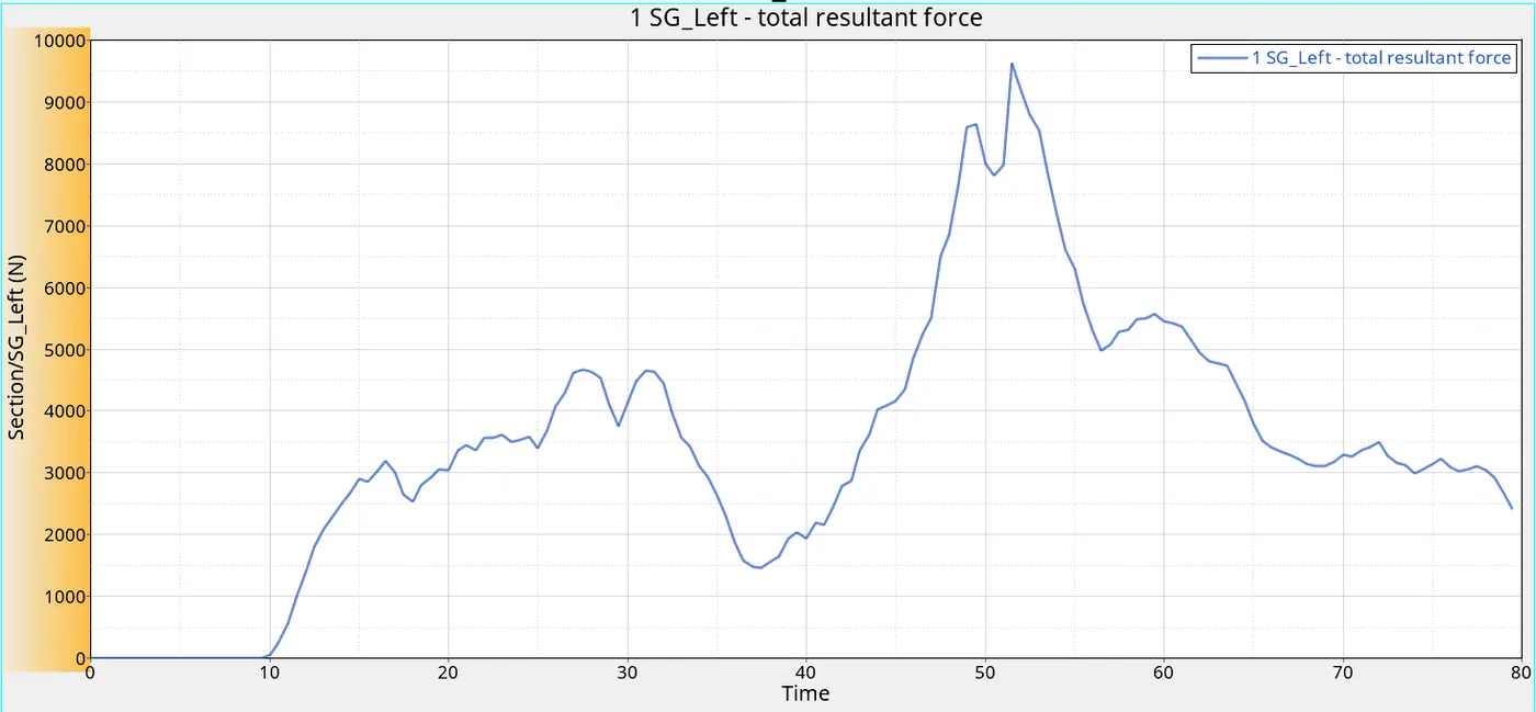
Plot 5: Time vs. Total Resultant Force (SG_Right) Plot 6: Time vs. Total Resultant Force (SG_Left)
| Sl No | Time (ms) | SG_Right Total Resultant Forces (N) | SG_Left Total Resultant Forces (N) |
| 1 | 0 | 0.00 (Min) (~9.526e-11) | 0.00 (Min) (~1.468e-08) |
| 2 | 9 | 0.3211 | 0.5266 |
| 3 | 10 | 116.708 | 52.042 |
| 4 | 29 | 4692.776 (Max) | 4108.346 |
| 5 | 50 | 2244.892 | 7996.358 |
| 6 | 51.5 | 2191.422 | 9632.694 (Max) |
| 7 | 79.5 | 4168.479 | 2419.095 |
Table 5: Time vs. Total Resultant Force (SG_Right) / Total Resultant Force (SG_Left)
The max total resultant force experienced at SG_Right= 4692.776 N
= 4.6927 KN at t=29ms
The max total resultant force experienced at SG_Left= 9632.647 N
= 9.632 KN at t=51.5ms
5. A pillar cross-section.
Follow the same steps from the previous case. Because of the high search distance, these areas are included as slave nodes at the beginning of the simulation. So we can record the changes in forces at the beginning of the collision. By analysing the plots, the maximum values of total resultant forces are different in both cases as well as the time. Like the previous case, the force is slightly higher in the left direction than in the right direction.
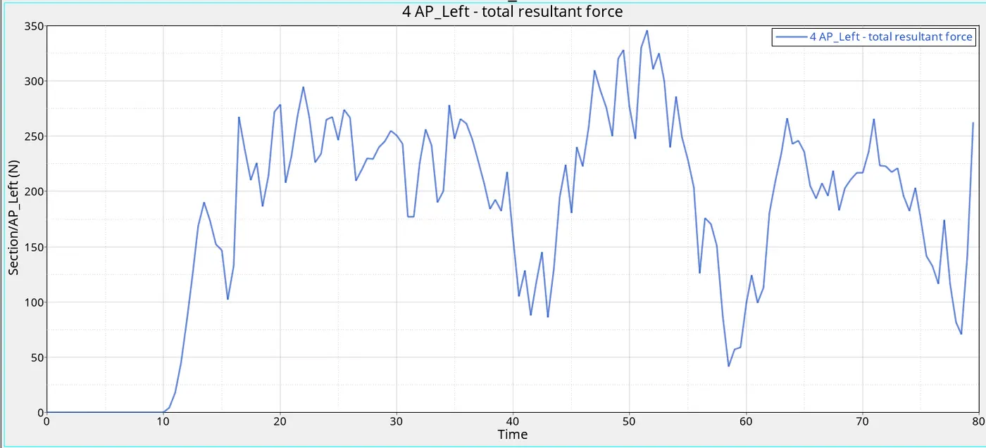
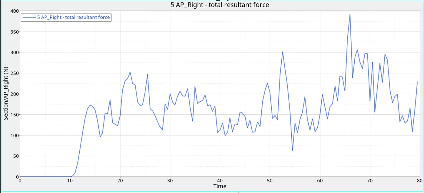
Plot 7: Time vs. Total Resultant Force (AP_Right) Plot 8: Time vs. Total Resultant Force (AP_Left)
| Sl No | Time (ms) | AP_Right Total Resultant Forces (N) | AP_Left Total Resultant Forces (N) |
| 1 | 0 | 0.00 (Min) | 0.00 (Min) |
| 2 | 9 | 2.987 e-05 | 8.827e-06 |
| 3 | 10 | 0.2195 | 0.2841 |
| 4 | 50 | 203.5005 | 248.089 |
| 5 | 51.5 | 137.441 | 346.029 (Max) |
| 6 | 66 | 392.709 (Max) | 0.1936 |
| 7 | 79.5 | 229.656 | 262.403 |
Table 6: Time vs. Total Resultant Force (AP_Right) / Total Resultant Force (AP_Left)
The max total resultant force experienced at AP_Right= 392.709 N
= 0.392 KN at t=66ms
The max total resultant force experienced at AP_Left= 346.029 N
= 0.346 KN at t=51.5ms
6. The axial force received on the rails from the bumper.
Like in previous cases, we have to plot and analyse the total resultant forces on the left and right rails.
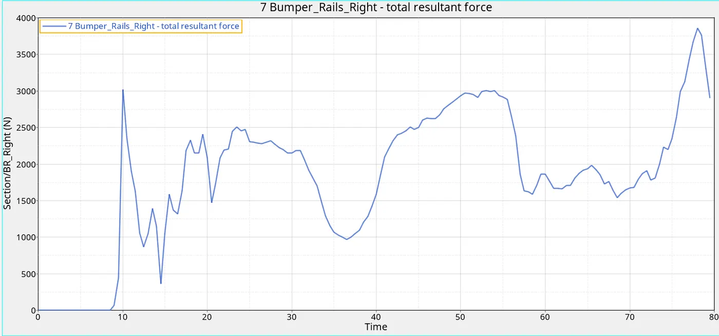
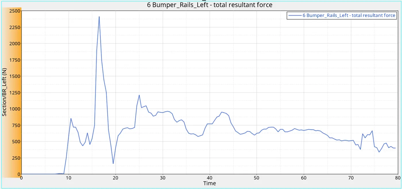
Plot 09: Time vs. Total Resultant Force (BR_Right) Plot 10: Time vs. Total Resultant Force (BR_Left)
| Sl No | Time (ms) | BR_Right Total Resultant Forces (N) | BR_Left Total Resultant Forces (N) |
| 1 | 0 | 0.00 (Min) (~1.611e-13) | 0.00 (Min) (~4.768e-17) |
| 2 | 6.5 | 3.2151e-8 | 0.00616 |
| 3 | 7.5 | 0.006541 | 3.593 |
| 4 | 8.5 | 0.00549 | 9.406 |
| 5 | 9 | 69.72 | 4.342 |
| 6 | 10 | 3019.847 | 590.750 |
| 7 | 14.5 | 359.78 | 452.165 |
| 8 | 16.5 | 1318.300 | 2411.2722 (Max) |
| 9 | 19.5 | 2408.197 | 160.8211 |
| 10 | 73 | 1807.86 | 552.622 |
| 11 | 78 | 3860.073 (Max) | 403.705 |
| 12 | 79.5 | 2904.09 | 400.696 |
Table 7: Time vs. Total Resultant Force (BR_Right) / Total Resultant Force (BR_Left)
The max total resultant force experienced at BR_Left = 2411.2722 N
= 2.411 KN at t=16.5ms
The maximum total resultant force experienced at BR_Right = 3860.073 N
= 3.86 KN at t=78ms
7. Acceleration curve received on the accelerometer at base of B pillar (on B pillar rocker).
Check the total resultant acceleration on each accelerometer. Both accelerometers come in the scenario after 13ms.
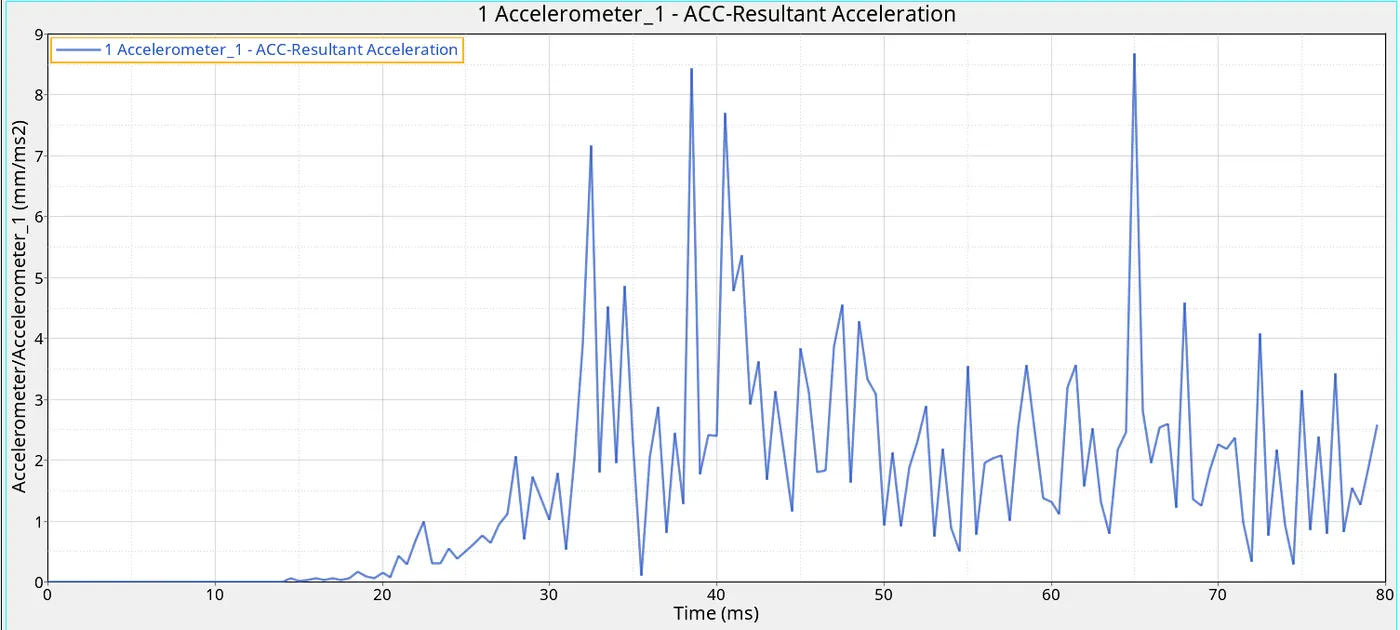
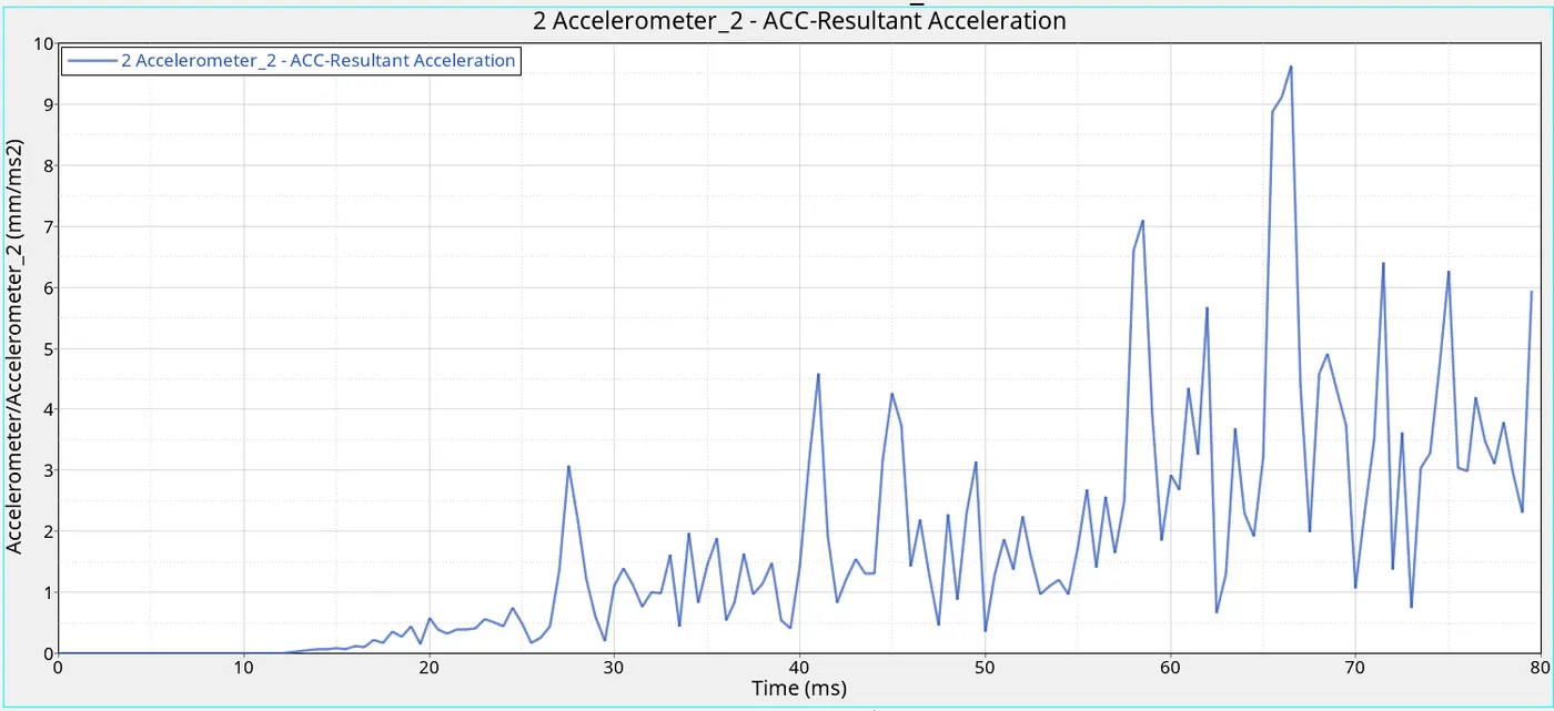
Plot 11: Time vs. Resultant Acceleration (Accelerometer_Right) Plot 12: Time vs. Resultant Acceleration (Accelerometer_Left)
| Sl No | Time (ms) | Accelerometer_Right (mm/ms2) | Accelerometer_Left (mm/ms2) |
| 1 | 0 | 0.00 (Min) | 0.00 (Min) |
| 2 | 13 | 0.00054 | 0.0271 |
| 3 | 32 | 3.916 | 1.009 |
| 4 | 32.5 | 7.167 | 0.984 |
| 5 | 63.5 | 0.799 | 3.689 |
| 6 | 65 | 8.667 (Max) | 3.209 |
| 7 | 66.5 | 2.537 | 9.622 (Max) |
| 8 | 79.5 | 2.580 | 5.994 |
Table 8: Time vs. Resultant Acceleration (Accelerometer_Right) / Resultant Acceleration (Accelerometer_Left)
The maximum value of acceleration recorded in the Accelerometer_1 = 8.667 mm/ms2 at t=65 ms
The maximum value of acceleration recorded in the Accelerometer_2 = 9.622 mm/ms2 at t=66.5 ms
8. Intrusions on the dash wall 66695,66244.
The intrusions of nodes 66695 and 66244 can be calculated from the total elongation of the spring connected to the specific node in the specific direction. The spring is less stiff.
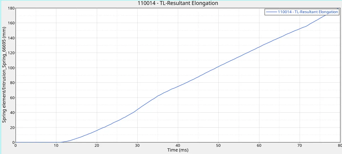
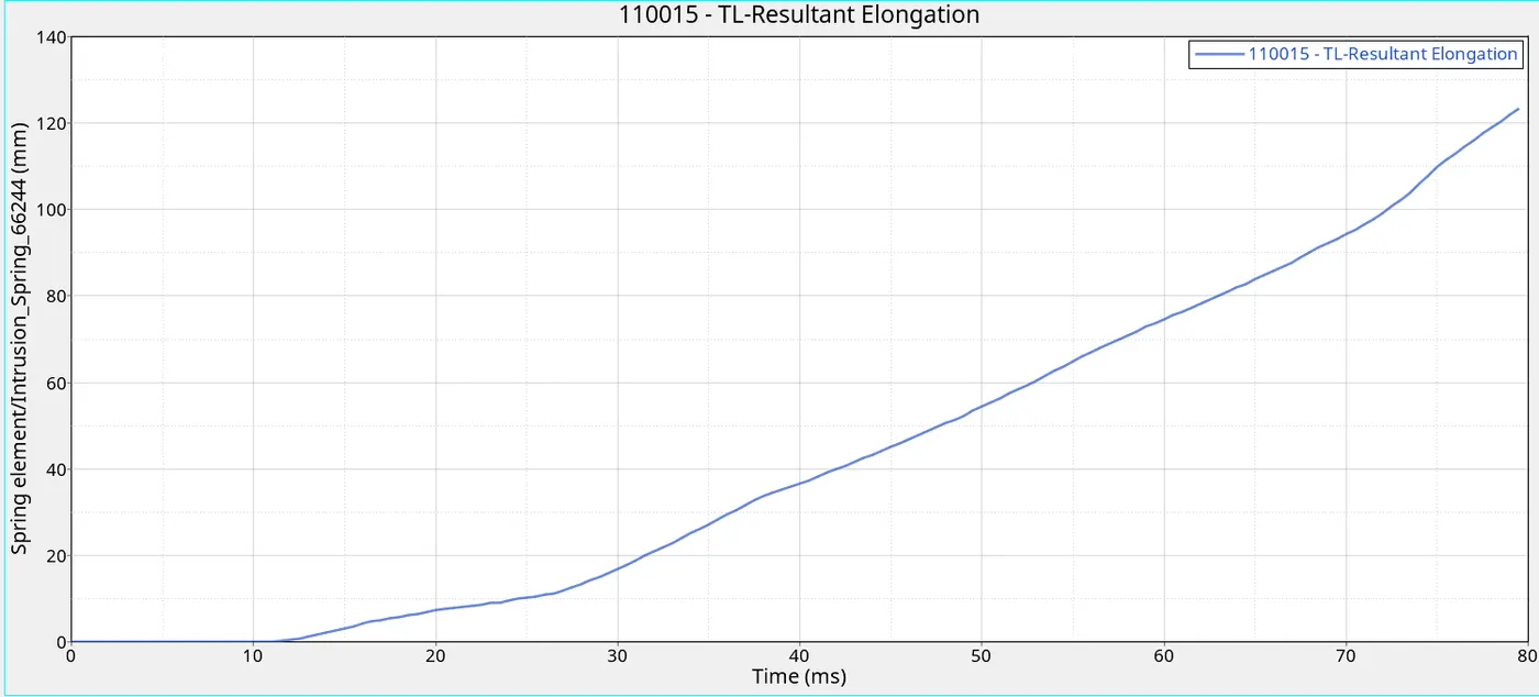
Plot 13: Time vs. Spring Element 66695_Total Elongation Plot 14: Time vs. Spring Element 66244_Total Elongation
| Sl No | Time (ms) | Spring Element 66695_Total Elongation (mm) | Spring Element 66244_Total Elongation (mm) |
| 1 | 0 | 0.00 (Min) | 0.00 (Min) |
| 2 | 7.5 | 0.00 | 0.00 |
| 3 | 8 | 5.957 | 6.48e-12 |
| 4 | 50 | 101.583 | 54.440 |
| 5 | 79.5 | 179.734 (Max) | 123.236 (Max) |
Table 9: Time vs. Spring Element 66695_Total Elongation / Spring Element 66244_Total Elongation
The max elongation of Spring Element 66695 = 173.734 mm at t=79.5 ms
The max elongation of Spring Element 66244 = 123.236 mm at t=79.5 ms
5. Results
- For the given model, simulate the crash scenario with the mentioned parameters and objectives and with the help of necessary plots, point out the outcomes and their values in the mentioned output requests.
Simulation File:
https://drive.google.com/drive/folders/1fxp6X8xqS7O-FbEXa_RVulyAHl0hgwON?usp=drive_link