Assignment 6-Frontal Crash Simulation Challenge

Title: Frontal Crash on BIW Model of DODGE NEON (FMVSS 208)

Objective: To observe the travel of force through various regions of the structure, check the crash pulse using accelerometer below B Piller Rocker position, etc using RADIOSS Solver.

Tools Used:

Hypermesh

RADIOSS

Hyperview

Hypergraph 2D

Procedure:

The give files are having two files (i.e 0000.rad and 0001.rad) 

The 0000.rad file has following information:

• Nodes
• Material Data
• Load Conditions
• Boundary Conditions

Basically the 0000.rad file contains all the model information. It is called as the starter file

The 0001.rad file which is know as Engine file. It holds all the necessary information about the simulation run. It contains

• Simulation Runtime
• Frequency of printing the output data such as number of time history files, animation files, etc
• The engine file is co-relation of the control cards used. Basically the engine file can be edited using the control cards.
• It always ends with 0001.rad

1. Verification of the Unit System.

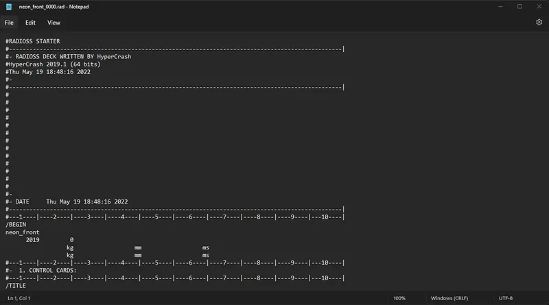
The given mesh model is verified with the consistent unit system. The model is imported in Hypercrash application and the units are checked. Another possible way is to check using the 0000.rad file of the model. It is opened in the Notepad and the block at the starting represents the unit system. The used Unit System for this analysis is kN kg mm ms. 

2. Penetration and Intersection check:

Penetration is defined as the overlap of the material thickness of shell elements, while intersection is defined as elements that actually pass through each other. All models and especially impact models should be checked for the penetrations and intersections and need ti be modified to ensure the model integrity. Penetrations affect the results. For eg due to presence of the penetrations there could be possibility of high contact forces and material plasticity eventually this may lead to sudden jumps in the energy plots. So initial penetrations should be removed. In order to check the penetrations in Hypercrash. 

Quality >>> Check Intersection on Tree >>> Select parts >> Click Check Penetrations

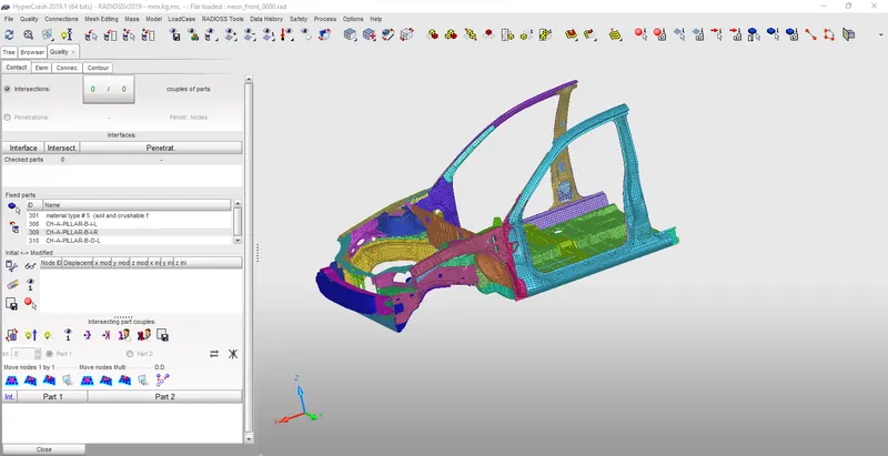
It can be seen that no any penetrations and intersections are present in the given model.

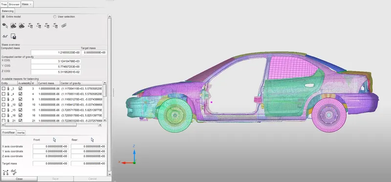
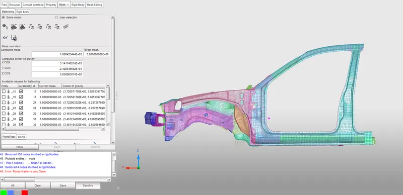
The next important task is to replicate the CG of the entire vehicle into the small model. The weight of the enitre vehicle is 1250kg approximately and the position of the CG is shown below. In order to replicate the mass and the CG position, some extra mass is added on some parts of the vehicle.

Vehicle's centre of gravity, or CG, is the imaginargy point where the sum of all the masses of each individual components effictively act. From physics perspective, if the CG is to high in Z axis of vehicle cordinate system it may cause roll over of the system while the CG at lower region is better for hadling of the vehicle as it reduces the weight transfered during the cornering and braking.

The mass is added using the rigid body. Two different regions are used, i.e one for the front end and the other for the rear end. In this way the total mass and the CG of the vehicle is replicated to the entire model of the vehicle.

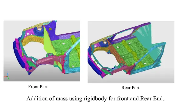
Following figure shows the CG of the half model. The position of the CG is at the same position as that of entire model.

3. Contact Interface:

In this model the TYPE7 contact interface type is used. It is a multi-usage impact interface, modelling contact between a master surface and a group of slave nodes. In this type there is also possibility to consider hear transfer and heat friction. 

The limitations of TYPE3 , 4 and 5 are solved in this type. The main limitation of this type is that time step is reduced at the high speed impacts. It also does not solve edge to edge contact. To solve this TYPE7 is used with TYPE11.

The TYPE7 interaction is called as Node to Surface contact type. Impact occur between a master surface and a set of slave nodes, similar to the TYPE5 interface. A node can impact one or more master segments and either side of a master segments. Each slave node can impact each master segment except if it is connected to this segment. A node can belong to a master surface and set of slave nodes. A node can impact the edge and corner of a master segment. This feature is not available in earlier interfaces. Recommended properties are as following

Igap = 2 (Variable Gap taken into account)

Gapmin >= 0.5 mm (minimum thickness to avoid the numerical issue)

Inacti=6 ( Remove initial penetrations wherever possible, else reduce to less than 30% of the defined gap)

Istf = 4 (Stiffness based on softer segment)

Stmin = 1 (Minimum stiffness in contact to avoid too soft contact )

Idel = 2 (Remove slave nodes from contact because of element deletion)

Iform = 2 (Frictional forces are calculated on the basis of stiffness parameter)

The existing contacts are deleted and new contacts are created with above recommended properties.

Apart from the entire structure a contact interface needs to be defined between the bumper and headlight component. As it is one of the objective to calculate the force transfered from the bumper to the headlight region.

For this contact the slave node is selected as bumper and the master component is selected as headlight with the recommended properties.

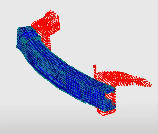
The red nodes are the slave part and the blue surfaces are the master part of the contact.

3. Rigid Wall 

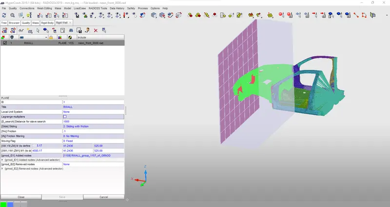
Rigid wall provides the contact between the rigid surface and nodal points of the deformable bodies. Rigid walls can be created with different shapes and size.

In order to define the Rigid wall using hypercrash go to Load Case >> Rigid Wall>> Plane Rigid wall. 

In properties give the proper name and select sliding with friction and give value of 0.1 for position of the wall select the tail and head of a vector using the nodes on the vehicle. This will define the Rigid Wall. For the distance of slave search enter the value of 1000. In this region the slave node will be selected. Apart from this the vehicle can also be selected as a seperate set of nodes to this rigid wall at the same time.

 4. Initial Velocity

As per the FMVSS standard 208 for the frontal crash the velocity of the vehicle is 35 mph (15.64 m/s). This velocity is constant before the crash with rigid wall. In order to apply the initial velocity in the Hypercrash. 

Load Case>> Initial Velocity and following window appears.

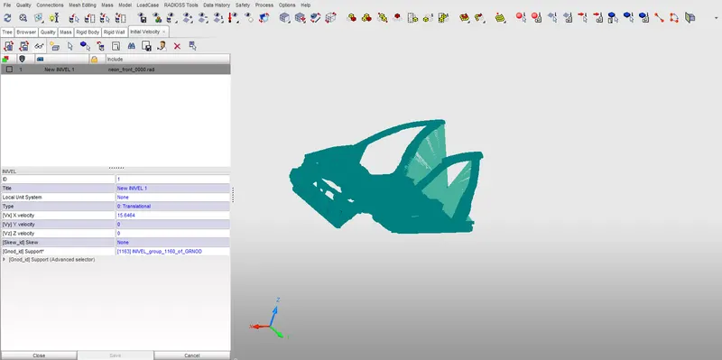
In the options, as the vehicle is moving along X axis the value is entered in the X component i.e 15.64 m/s. In the Support all the nodes of the vehicle are selected. 

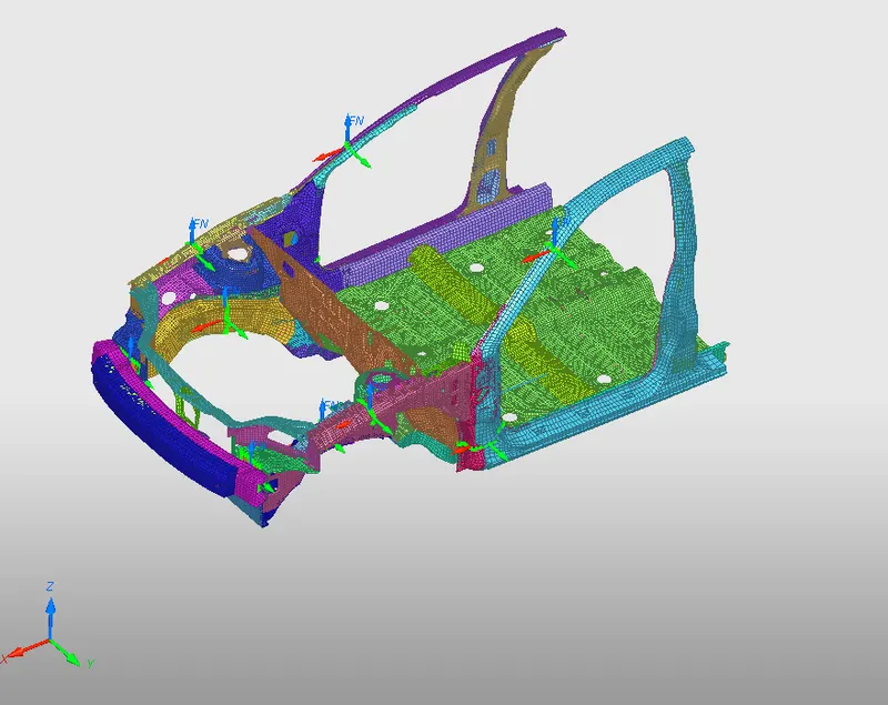
5. One of the deliverable is the sectional forces at the given locations. It is important to understand how to extract the sectional forces. In this work the sections are created at A-Pillar, Shot Gun, Rails and the Bumper. It is of high interest to know how the forces are transmitted from the Bumper to the Dashboard and the rate of deformation for the safety of the passenger.

The reason for determining the forces is that, certain components have to crash more than the other components, so that the forces are distributed correctly and leaving very less forces entering into the cabin.

Hence it is of high interest to determine the forces at the Left and Ride side of the vehicle at Rail, Shotgun and A Biller, Fender and hinge pillar. 

Following is the procedure for setting up the section in Hypercrash.

Data History >> Section >> New Section >> Default sections and then following window appears.

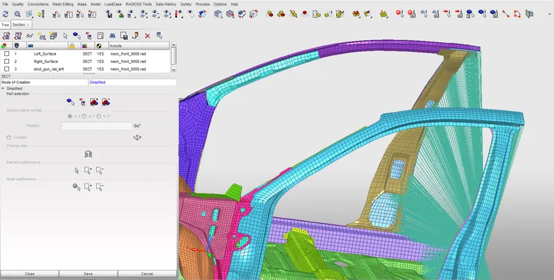
The component is selected at which the section is interested. Next the nodes and element are selected such that the coordinate system is defined to get the force oreintation. The data of the forces is by default recorded in the Time History section.

Following figure shows the position of all the desirable sections.

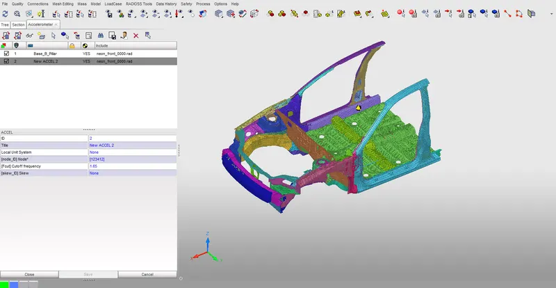
The next important is to setup the accelerometer at the desirable positions. An accelerometer is a electromechanical device that measures acceleration forces caused by gravity or motion. It is basically converting the mechanical motion into an electrical signal.

To create accelerometer in hypercrash click Data History >> Accelerometer >> New Accelerometer. In the options select the node at which the accelerometer should be placed. In this simulation the area of interest is at the base of B pillar. For the coordinate system keep the default other unit system can be created if required. And the cut off frequency of 1.65 is kept as default.

 The next interested ouput desirable is the intrutions in the compartment of the vehicle. For this there are two possible ways to calculate these intrutions. One method is to create a spring with very low stiffness value and extract the deformation of the spring. Second is to record the time history of the node with a moving frame at certain location. In this study both the methods are implemented to see the results from both the approach.

First it is explained with respect to the spring method.

 Go to Mesh Editing >> Element >> Create >> New Part >> Type Spring >> Select the property for spring >> Select the nodes between which the spring is created 

The property card for the spring is /PROP/SPRING. The following figure shows the used setting for the spring property card.

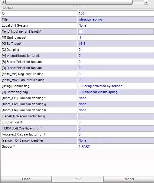
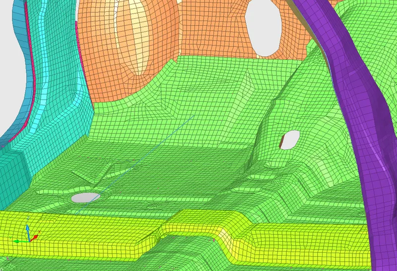
 As it can be seen that the mass and the stiffness of the spring are kept to very low value. Following figure shows the spring connected between the nodes of interest.

The second method is by tracking the node with respect to a moving fram so that the deformation of the cabin can be recorded. So for this the Moving frame is to be created initially.

Go to Radioss Tools >> Skew/Frame >> Create new >> Select Frame and in the options select the Moving Frame. For defination of the XY plane define using the nodes. In this way the Frame is defined.

So in the next step the node history is to be requested to get the interested variable for the node.

Go to Data History >> Time History >> Create >> TH of Node

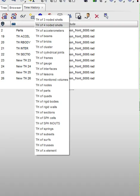
In the variable box select the desirable output variables to be extracted. In the Node box select the nodes for which the Time history is to be extracted. Here addition to the nodes it is also important to define the Frame defined in earlier step. It is important to note that no node can be repeated in single defination. A new time history object can be used in such case. 

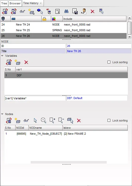
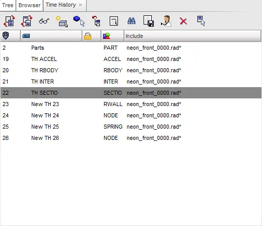
The accelerometer placed at the base of the B Pillar also needs to be added to the time history and additional to this the sections, spring and the Interfaces created earlier also needs to be added in the Time History.

Output Request	Position
INTERFACE	Left and Right Bumper and headlight
ACCELEROMETER	Left and Right base of B Pillar
SPRING	Intrusions on node 66244 and 66695
SECTION	Left Rail, Right Rail, Left and Right A pillar, Left and Right Shotgun
RWALL	Rigid Wall

6. Setting up the Control Cards. 

As defined earlier the starter file checks the errors in the model and engine file is which simulates the model based on the requested card setttings. So engine file is the one  which produces the necessary output. 

a. DT_ELTYPE_KEYWORDIFLAG

This is used to set up the Nodal Time step of 0.0005ms. To refrain from numerical instability, the scale factor is set to 0.67, which ensures the analysis doesn't fall into instability.

b. RUN

This card helps to set the total run time of the simulation which is set to 80ms. 

And various other basic cards such as ANIM_DT, ANIM_MASS, TH are used.

7. Model Checker and Penetration Check

After setting up the entire simulation model. A penetration check is performed, to confirm that no any nodes or elements are penetrating, if certain are penetrating they are removed using the possible options like Moving the node.

The Model checker is also deployed after the penetration check. This gives the warnings and errors in the model definition, boundary conditions, interfaces, kinematic conditions, etc.

After this, the file is run through the Radioss Solver option in Hypermesh. 

The model is imported in Hypermesh with Radioss profile and it is submitted for the run.

Post Processing:

For the post processing Hyperview is used to visualize the animation result files and hyperplot for plotting the required graphs.

Animations

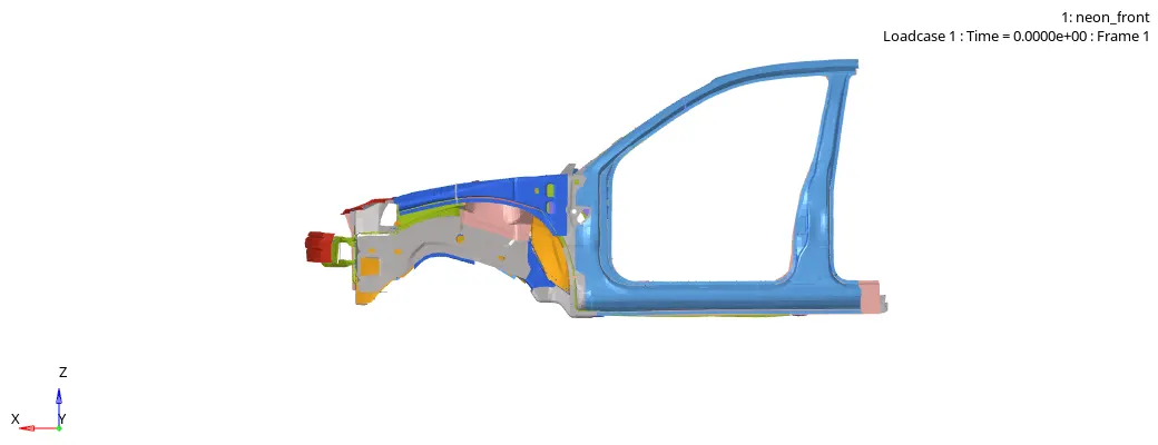
a. Crushing of the BIW

b. Von Misses Stress Animation of the BIW

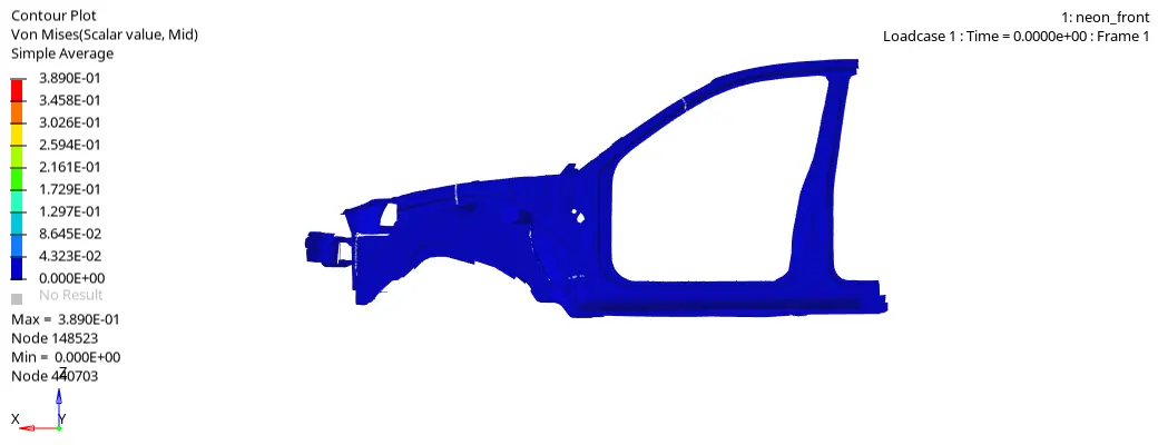
From the animation result of the BIW it is clear that the structure is crushing in a sequence where initially the bumper starts crushing, after the complete absorption of the energy by the bumper the forces start to transfer to the rails, which in turn starts to absorb the energy. After the deformation of the rails the forces are transferred to the A pillar. It can be seen that after approximately 45ms the A pillar starts to buckle. So the transmission of the forces is occuring as per the required path, i.e Bumper to Rails to A pillar. In each phase the force willbe reduced as the energy absorbtion occurs in each phase.

Global Energies and Mass Error:

a. Energy and Mass error

The energy and mass error of the simulations give an idea about the acceptability of the results. High Mass and energy error results may lead to false results. As issue such as Hourglass, time step, etc may lead to high errors.

In order to check the mass and energy error, 0001.out file of the simulation is opened. In this file the energy and mass error is printed.

 

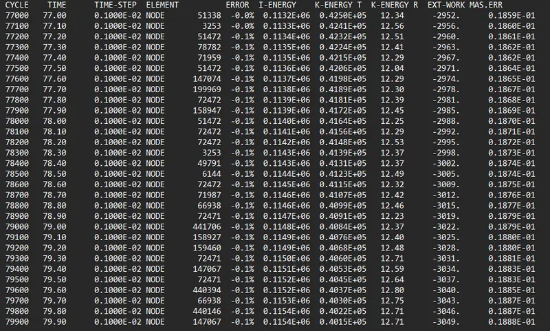
It can be seen that the energy error at the end of the simulation is around -0.1% and for mass error it is around 1.88 %, both the values are way below than the acceptable values. Hence the results of this simulation are acceptable.

Generally the under integrated elements( Belytschko shells, solids with 1 integration point), the hourglass energy explains the negative energy and it is not counted in the energy balance. The normal amount of Hourglass energy is about 10 to 15 %. Higher amount of positive energy may be due to the incompatible kinematic conditions, such issues need to be identified. 

b. Plots for Kinetic, Internal and Total Energy

The plots for the Kinetic Energy, Total Energy, Internal energy and Hourglass energy will give an idea of the conservation of the energy in the simulation. Following plot shows the Kinetic energy, Internal Energy, Hourglass and Total Energy of the system with respect to the run time.

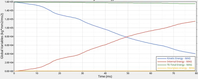
As the fundamental law of conservation of energy says that Energy can neither be created nor be destroyed but can be converted from one form to another. As the BIW is moving with initial it possess high Kinetic Energy as it impacts with the rigid wall, the energy is absorbed by the components of the BIW, hence the KE is converted into IE.

As the elements used in the simulation are of improved intergrated elements, there is almost zero Hourglass energy in the system. Ideally the KE should be entirely converted into IE. But Hourglass and contact energies can occur in the system which are not accounted for the Total energy equation. Hence in this run there is very negligible loss of energy which was earlier discussed.

Sectional Forces:

a. Sectional Forces in Rail

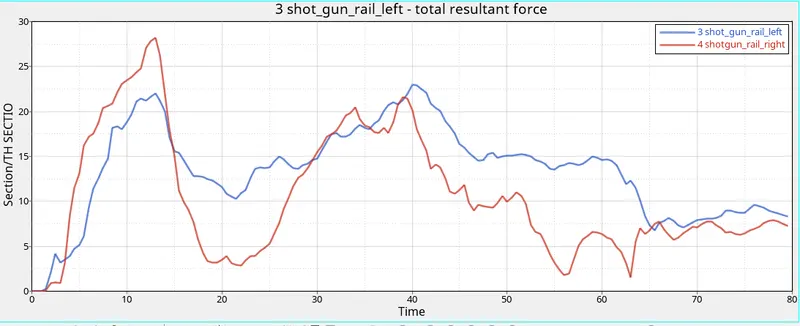
The maximum rail forces at the Left rail is 23N and for the right is 28N. The peak is observed at the 12ms of the run time. The first peak occurs when the stiffness of the rail is high enough to resist the force and after 12ms it starts to deform. The second peak occurs at 40ms at time when the section is already in contact with the rigid wall.

b. Fender Sectional Forces

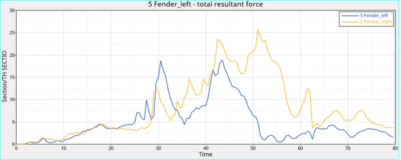
The maximum forces in the left fender is 20N where as for the right is 25N. The peaks occur at different time is due to the position of the sections and the values of the peak are due to the deformation characteristic of the model at that position.

c. Section forces at A Pillar

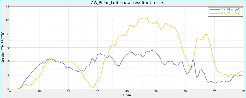
The maximum values for the A Pillar left is 6N whereas for the right A Pillar is 10N. Both the peaks occur at apprx. 40ms. In the inital phase of the crash, the bumper and rails are in contact with the rigid wall absorbing energy and hence lower values of forces at the A pillar are seen. Once the deformation of the rail and bumper is completed the A pillar expierences high value of forces.

d. Intrusions in the passenger compartment:

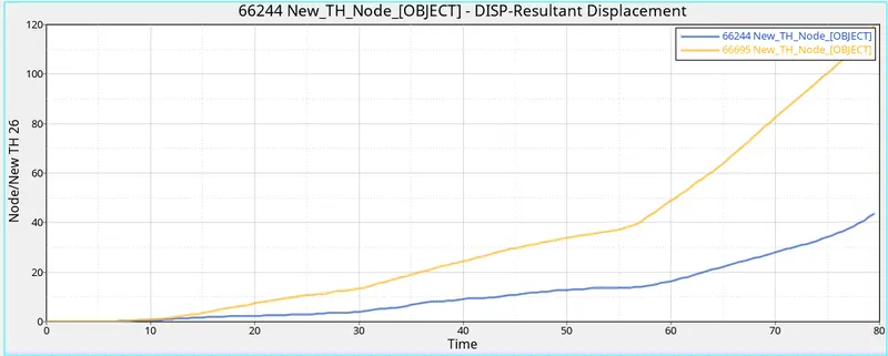
To check the intrusions at the dashboard of the passenger compartment. The output for the nodes (66695 and 66244) are extracted with respect to moving frame reference. The resultant deformation is plotted. It is seen that the maximum values are 120 and 42  for nodes 66695 and 66244 respectively. As the elongation is below the accepted value, it can be concluded that the fewer injuries will occur to the passenger/driver.

e. Accelerometer

Acceleration is the change of velocity w.r.t time. This curve gives the crash pulse of the crash. The acceleration at the base of the B pillar is recorded on both the sides. As the B pillar is located at good distance where the automobile is in contact with the rigid wall, which prevents the noise in the data. Following plot gives the acceleration curve,

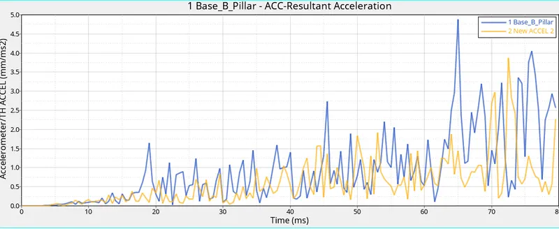
It can be seen that before the wall touches the car, the acceleration is constant. As soon as it touches the wall, the decelerration starts. With respect to time the rear part of the vehichle slows down later in corresponding to front part, which decelerates first. The sudden peaks are suspected due to the vibrations at the position of the accelerometer.

f. Forces from Bumper to Rail:

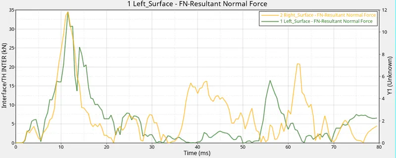
To record the forces transmitted from the bumper to rail, the output request for the interface between the bumper and rail is placed. The above graph shows the resultant normal forces for the interaction. The maximum value is around 35 KN. Initially there is low forces and once the bumper deformes, the strain energy is transfered to the rails.

Conclusion:

The Frontal Crash was performed on BIW Dodge Neon model as per the FMVSS 208, the simulation was performed importantly to check them;

a. How much of the Internal Energy is a vehicle able to absorb during a crash.

b. The deformation and forces at the critical areas. Most importantly to observe the force flow.

c. Occupant Safety

These parameters are compared with the Standard and its conclude how safe the structure is.