Assignment 6-Frontal Crash Simulation Challenge

Aim:To run a simulation for the frontal crash [BIW] and to obtain a results in the post processing.

Objective:

• To check the unit system in the solver.
• To create an appropriate interface,friction 0.2 and recommended parameters.
• To check for the penetrations and intersections.
• To create rigid wall with a freiction 0.1.
• To add extra mass attain a target mass of 700kg.
• To apply initial velocity to the car.
• To create sections and find sectional force in the rail,bumber,shotgun,A pillar.
• To create spring elements to get intrusions and to calculate the intrusions.
• To create accelerometer to calculate acceleration of the car.
• To create TH for all the inputs requested.
• To run the simulation.
• To plot graphs in the post processing.

Theoretical Framework:

• Frontal impact is performd at 64kph,the car crashes into a deformable barrier with 40% of its width front on the driver side.Readings takn from the crash test dummies are used to asses protection given to adult occupants in the front seat.
• Each car test is subjected to an offset impact into an immovable black fitted with a deformable aluminium honeycomb force.
• This impact is intended to replicate the effect caused in the car when crashing 55km/h 50% offset frontal crash with a similar mass car.As most frontal crashes involve only part of each car's front,the test is offset to replicate a half width frontal impact between two cars.
• In the test,this is replicated by having 40 percent of the width of the car crashing into aluminium deformable barrier.This represents the most frequent type of road crash,resulting in serious or fatal injury.
• The barrier face is deformable to represent the deformable nature o the cars.Two adult dummies are placed representing averahe sixe men in the driver's seat and front passenger and two children,aged 18 months and 3 year old,on child retraint systems are placed in the rear seat.
• Contact between the occupant and hard intruding parts of the passenger compartment is the main cause of serious and fatal injuries for restrained adult car occupants.
• The test speed of 64km/h represents a car to car collision with each car travellig at around km/h and crashing % of their width.
• The difference in speed is due to the energy absorbed by the deformable face.Accident research has shown that this impact speed covers a significant proportion of serious and fatal accidents.
• By preventing intrusion,the chances of the occupant impacting the car's interior is minimised with space remaining for the retraint system to operate effectively.Steering wheel and dashboard mounted airbags are an important part of the driver's restraint syatem.

  

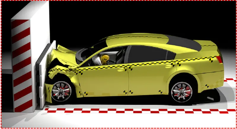
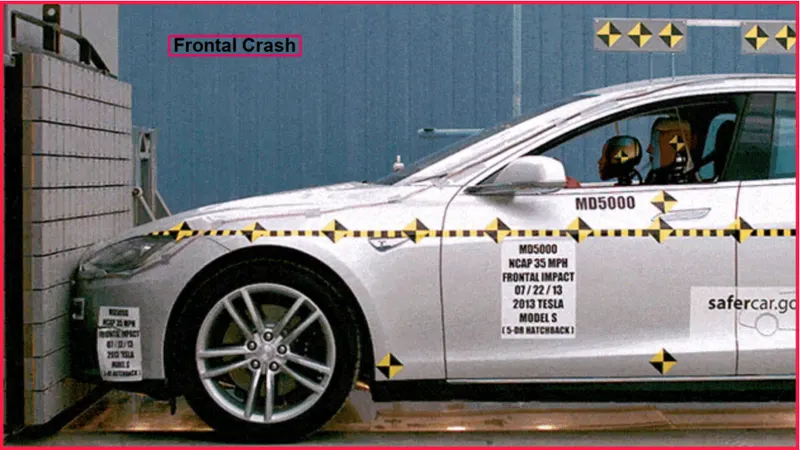
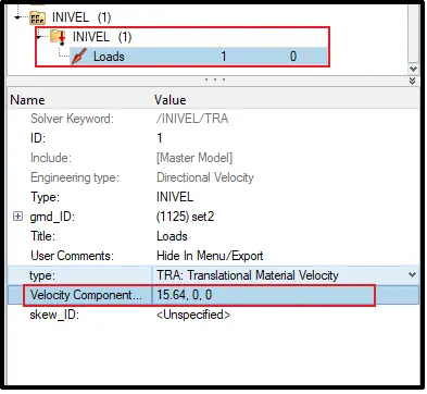
[Note: According to FMVSS{Federal motor vehicle safety standards}. Assign a inital velocity of 35mph,1mph=0.44704m/s,=35x0.4470=15.6464m/s.

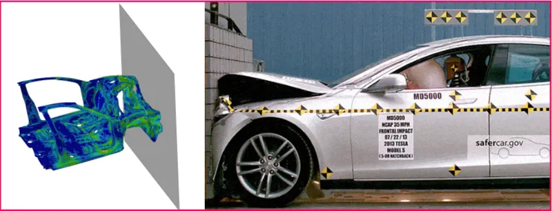
Procedure:

Phase 1- Check unit system and either follow [Mg mm s] or [Kg mm ms]

• While opening hypermesh software,A user profile window will pop up,switch to the radioss user profile as shown in below figure and start importing the model into the solver deck.

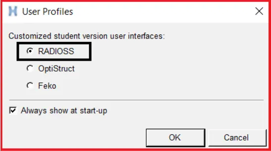
• Now after switch the user profile to radioss,import the model into the radioss solver deck.
• To import the model,go to standard panel>>import>>import solver deck.

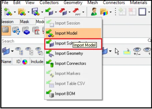
• Import solver deck option should be selected to import the radioss starter file.

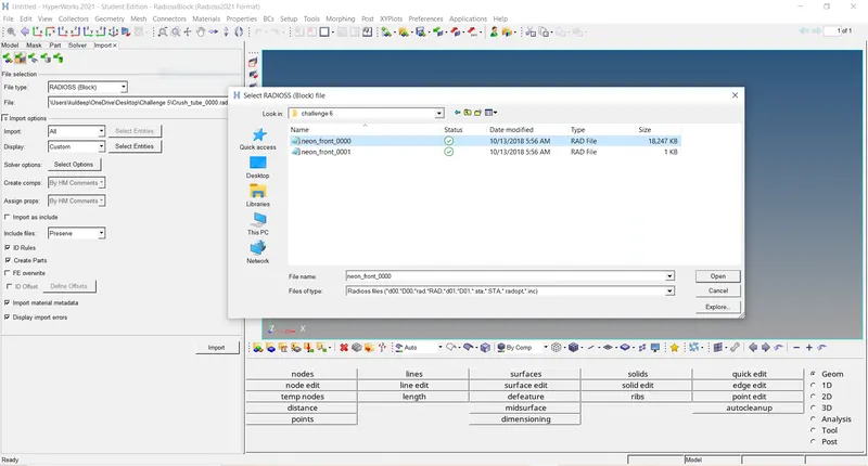
• Here the import browser will appear as shown in above fig,select the appropriate starter file to import into GUI.
• Switch the file type to radioss block and import the model into GUI.

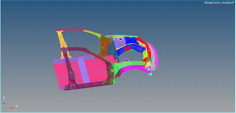
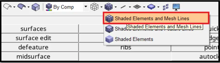
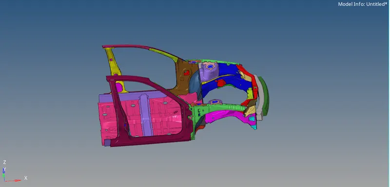
• Here the model is in wireframe mode,switch to the shaed mode as shwon in below fig.
• To switch to shaded model,go to visualization tab>>shaded elements and mesh lines.

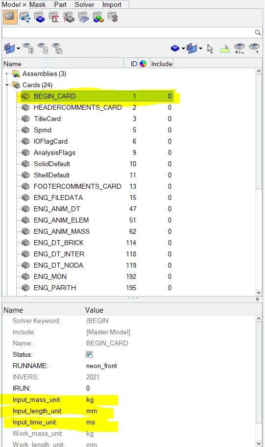
• Now go and check for the unit system of the model.To check for the unit system,go to the model browser>>control cards>> BEGIN_CARD.
• Check for the unit system is shown in below fig.

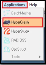
• Now go to the hypercrash,to go,go to the Menu bar>>application>>hypercrash.which is shown in below fig.

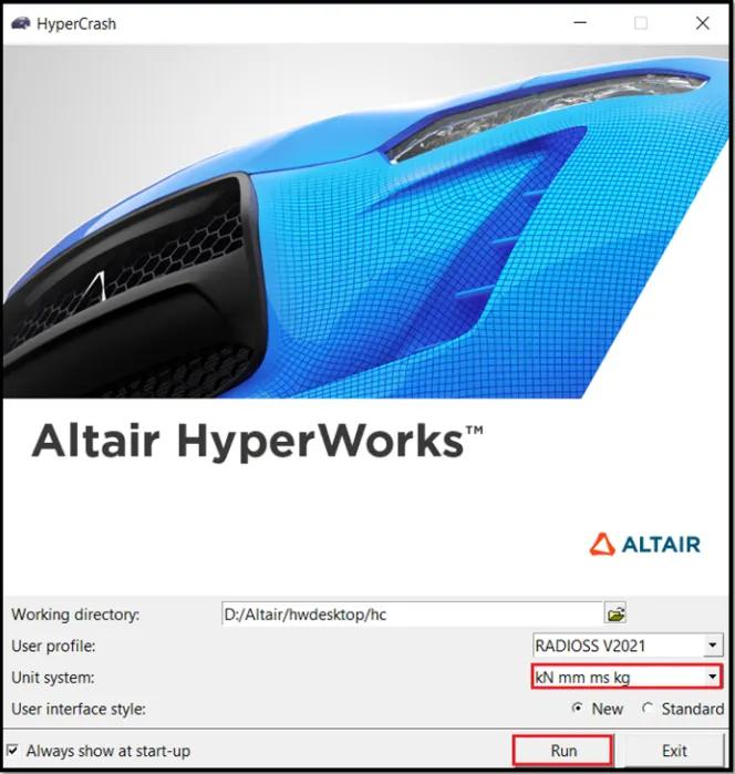
• Make sure whether the unit system in hypermesh is [KN,KG,MM,MS],Which is shown in below fig.

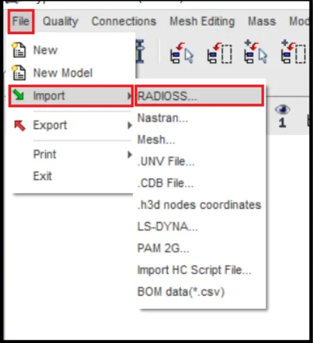
• Now import the model in hypercrash,to import the model,go to menu bar>>file>>import>>radioss,which is shown in below fig.

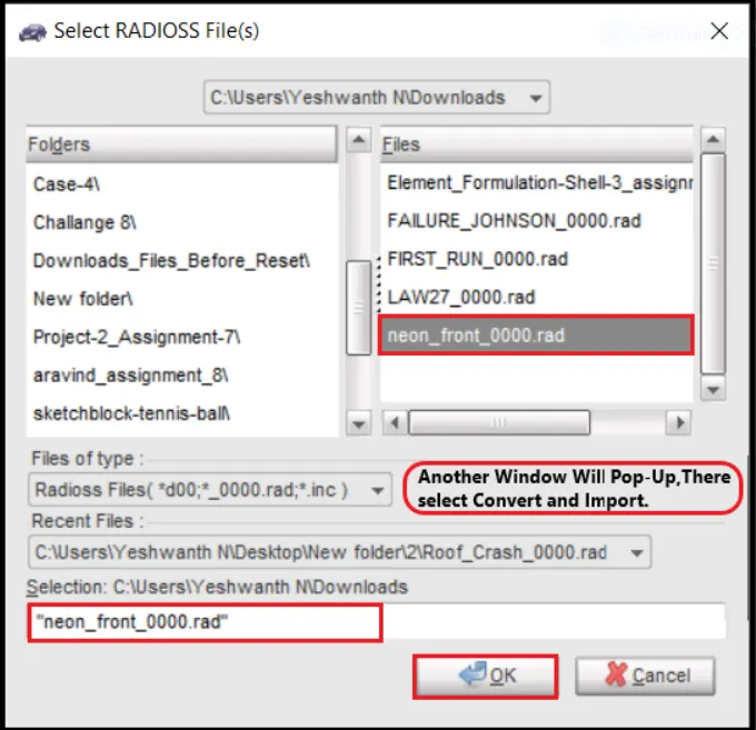
• Here select the appropriate radioss file and import the model into hypercrash,which is shown in below fig.

Phase 2- Mass balancing [Adding mass to the model to get COG at proper poasition]

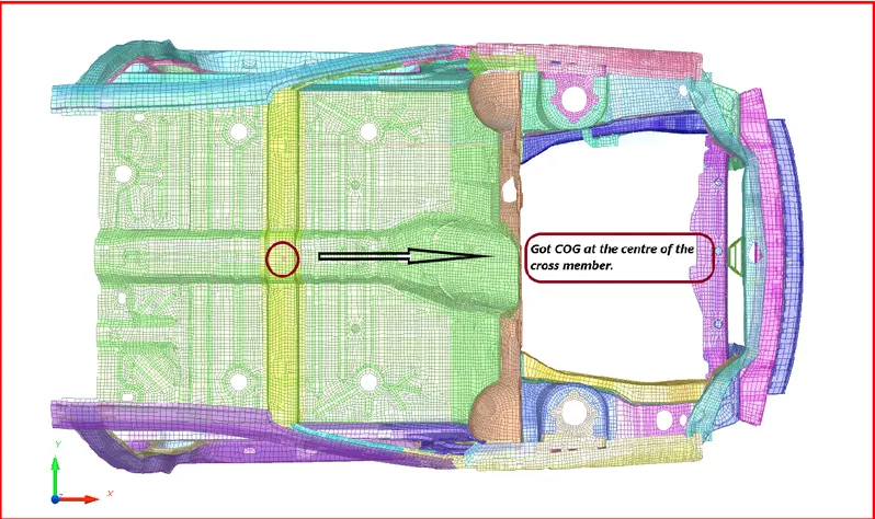
• Here the COG is not in proper position which is shown in below fig,so we need to add mass to get COG at proper position.Its like balancing.
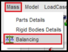
• To check the mass and COG [Centre of gravity],Go to hypercrash menu bar>>mass>>balancing,which is shown in below fig.

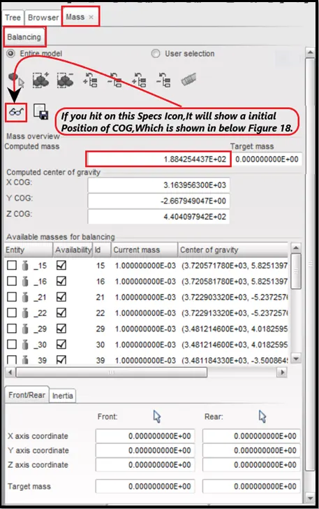
• After hitting on the icon which is shown in below fig,The initail poaition of COG will appear which is shown in below fig.

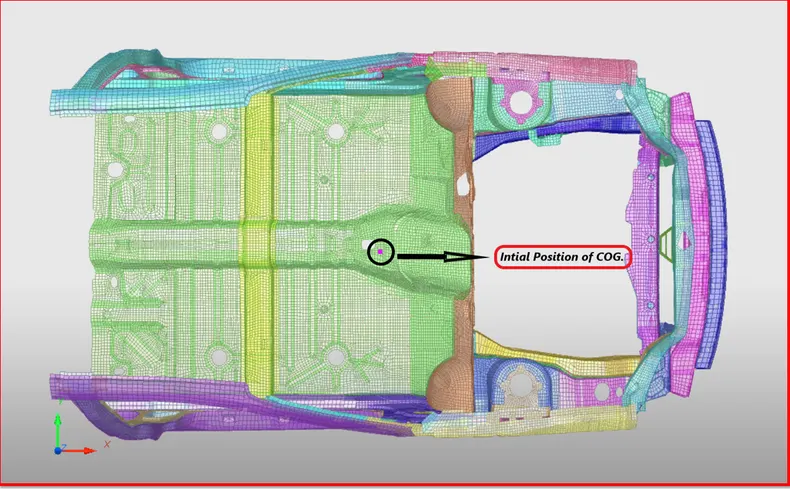
• Now mass should be added to get COG in proper position.It should be in centre of the cross member.
• To bring COG to the centre of the cross memeber,we should add a mass.
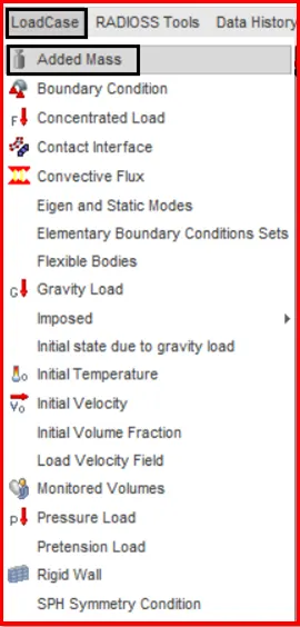
• To add mass, go to load case>>added mass.Which is shown in below fig.

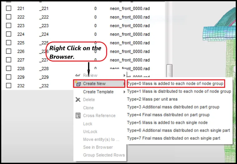
• Now right click on the added mass browser and select TYPE=0 where the mass will be added to every single node,which is shown in below fig.

   

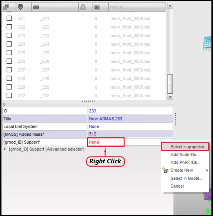
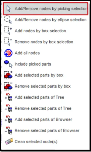
• Here right click on the [grnod_ID] support to pick the nodes to add mass,which is shown in above fig.

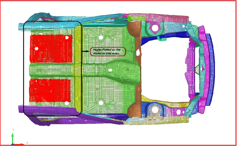
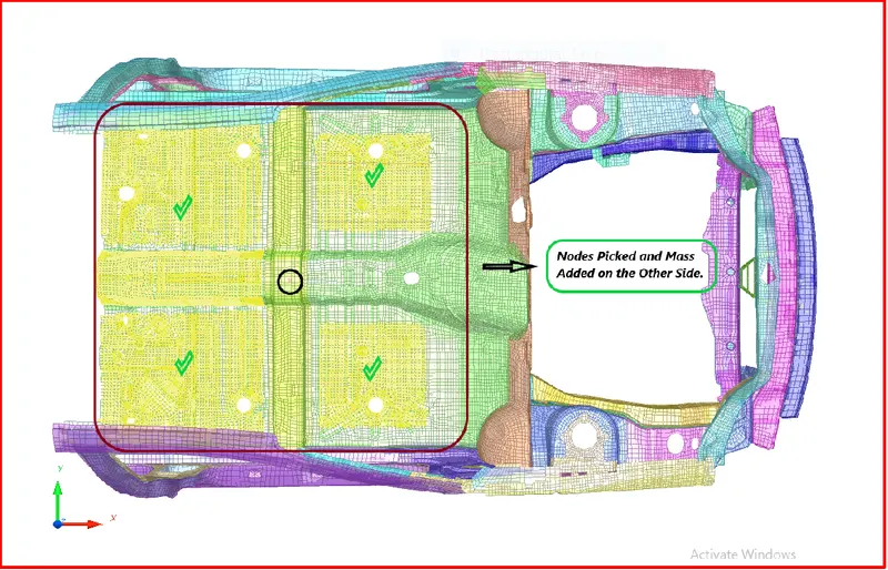
• Here in the above fig.The nodes were picked on the model to add mass.

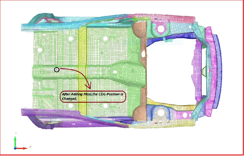
• Here after adding mass on the nodes,The COG position is changed which is shown in above fig.

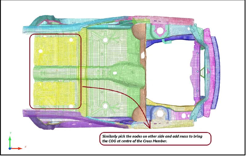
• Here,similarly pick the nodes on the other side of the model and add mass to bring the COG at centre of the cross-member.

• The nodes have been picked and mass added to the other side of the model,which is shown in below fig.

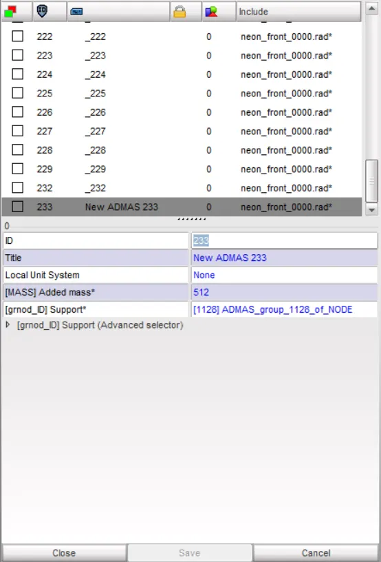
• We have attained the mass by adding the mass to the nodes,which is shown in below fig.

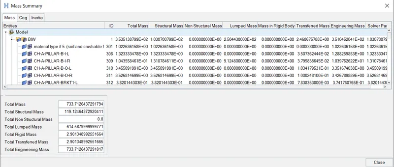
• Now export this file and save it in a specified location and import this model into hpermesh and check the total mass.

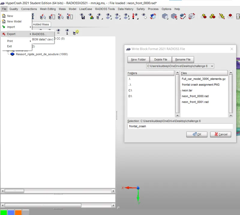
• Now import the exported model from hypercrash to the hypermesh.

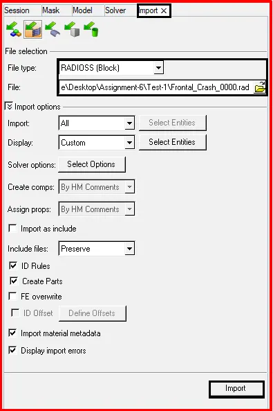
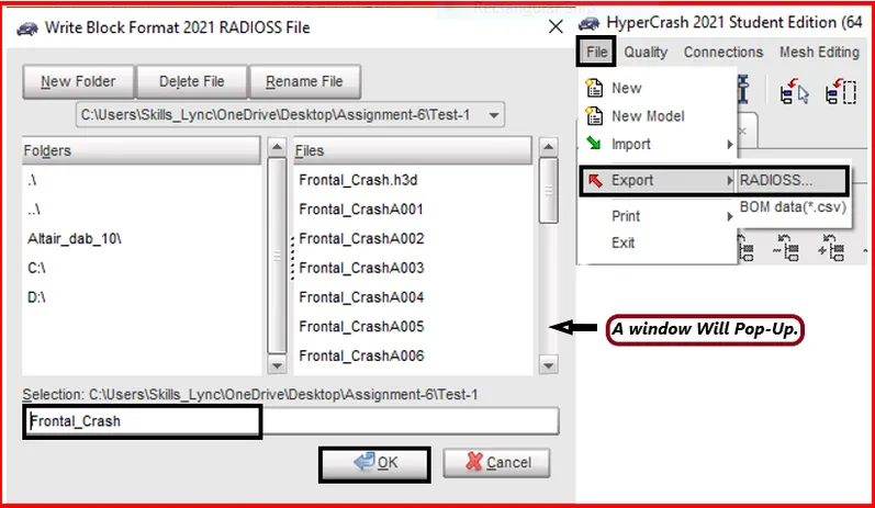
• Next go and check in hypermesh,whether the we have attained 700kg mass.
• To check, Go to menu bar>>tools>>mass details>>mass, COG, Inertia.Which is shown in below fig.

Phase 3- Check for the Penetration:

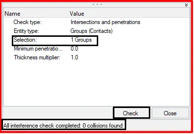
• Here check for the penetration,to check go to menu bar>>tools>>penetration check.Which is shown in below fig.

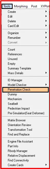
• Next select the groups [Interfaces] to define,which is shown in below fig.
• Then click on the check to check penetrations in model.If the penetration exist,it throw a error in the status bar,if the penetration does not exist,it will display No collision found which is shown in below fig.

Phase 4- Create the interfaces:

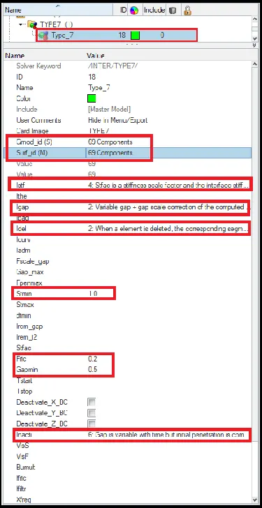
• Here for this model.TYPE7 contact interface is created with the recommended parameters,which is shown in below fig.

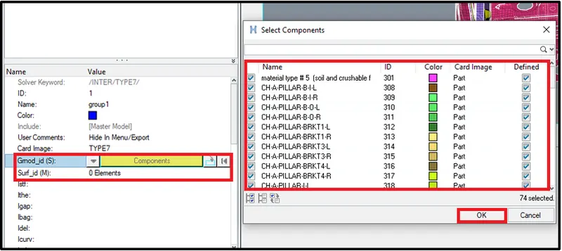
• Select the slave and master nodes by switching to the components and select all the componenets for slave and master nodes which is shown in bwlow fig.

Phase 5- Creation of sections:

• Here we have to create a section,the section should be created at the node.
• To find we have to display the numbers in the display panel,which is shown in below fig.

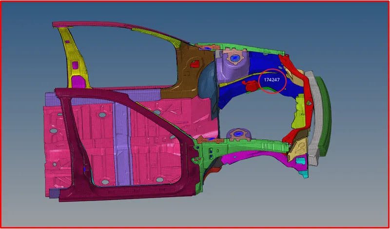
• Select the node by ID and enter the ID number and click on which is shown in below fig,the node number will be displayed,we have to create a section there.

• The node number is displayed,which is shown in below fig.

• Next for creating section,we need frame,so we need to create frame first.To create frame right click on the solver browser>>create>>frame>>mov.which is shown in below fig.

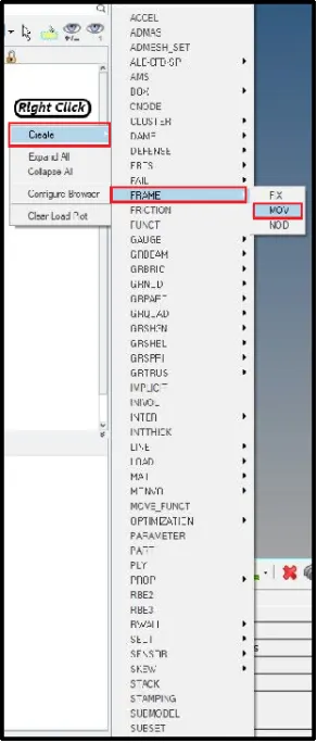
• Next select the nodes to specify the location of the frame to be created on the model.
• Switch to the create by node reference,now select the node at origin>>node at Z-axix>>Node at YZ Plane,which is shown in below fig.

• The nodes selected to be created to create a frame at a specified location is shown below fig.

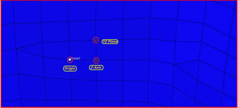
• The frame created is shown in below fig.

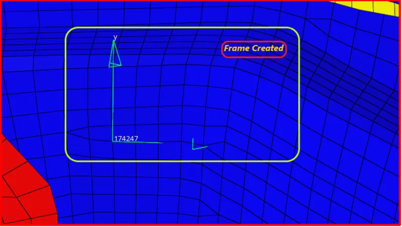
• Then create a section,to create a section,right click on the solver browser>>SECT>>SECT,which is shown in below fig

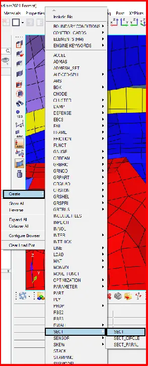
• After selecting the SECT to create section,A parameter window will be opened left side.
• There will be nodes [N1,N2,N3] Select the nodes to create a section,which is shown in below fig.

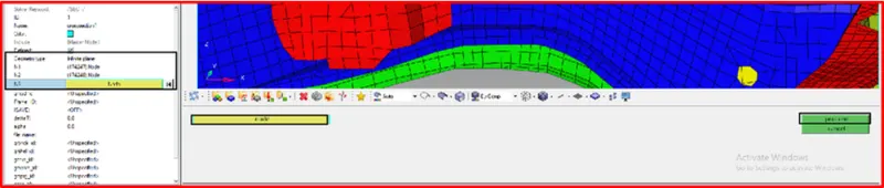
• Next select the frame ID,which is shown in below fig.

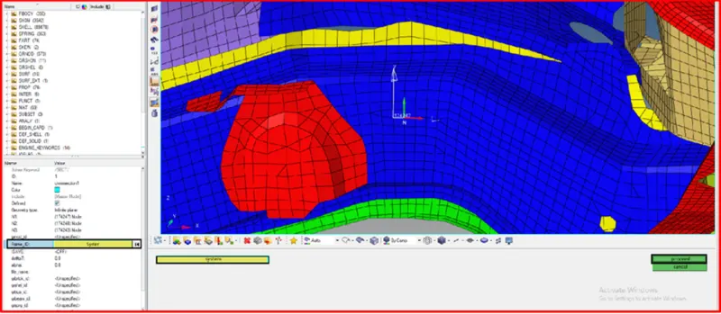
• Next right click on the grshell_id to select the elements,where we created the section,which is shown in below fig.
• Enter the values for delta and alpha.
• Coefficient of filtering (alpha=0.67)
• Time step for saving the data (deltaT=0.001)

    

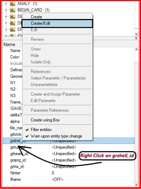
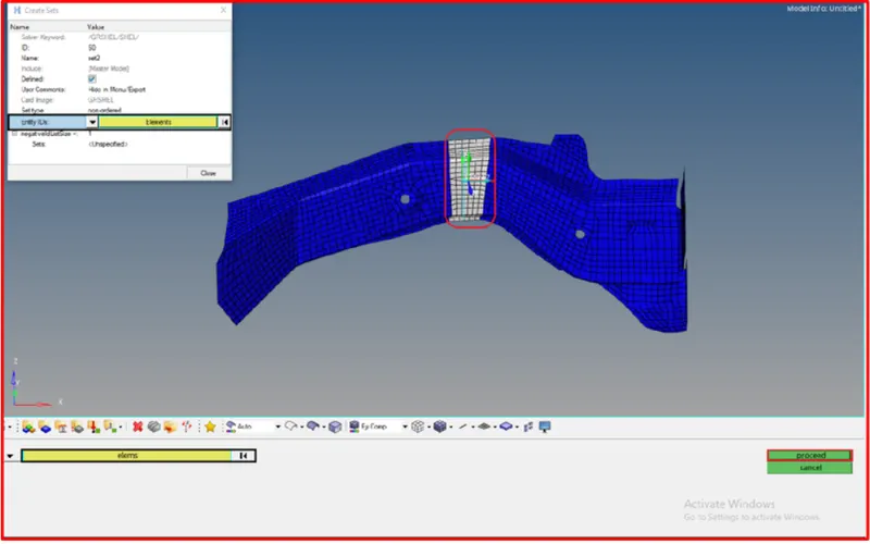
• Every parameters have been specified which is shown in below fig.

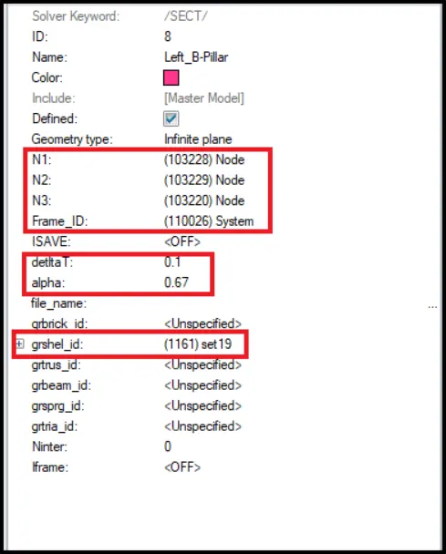
• A section has been created which is shown in below fig.

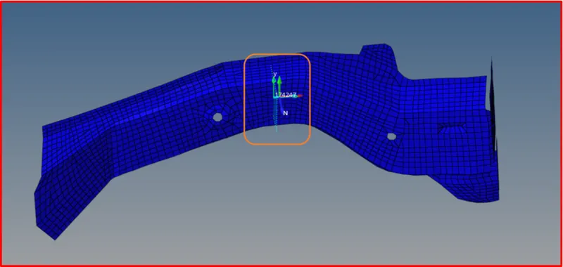
• Now we have to check whether the section created for the rail componenet is fine or not.
• If all the nodes get realized in the elements,then the section created for rail componenet is fine,which is shown in below fig.
• A one row of elements should be maintained.
• To check,right click on the section in the model browser>>review.

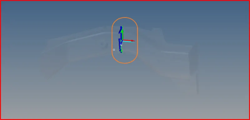
• Similarly,we have to create a section in the other side.
• For that,create a temp node at 174247 node and translate the node to the other side and create a frame and section which is shown in below fig.
• To create a temp node,go to geometry>>temp node>>select the node at the required location>>add.Which is shown in below fig.

• The temp node is created which is shown in below fig.

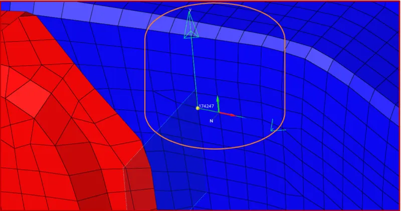
• Now translate that node to other rail componenet.
• To translate,go to tools>>translate>>select the node and make it as duplicate and translate>>switch to the Y-axis>>Magnitude>>Translate.

• To bring the one particular component individually,press D which is called display and select the componenet,which we want to bring it individually and press reverse.
• The componenet will be brought individually which is shown in below fig.

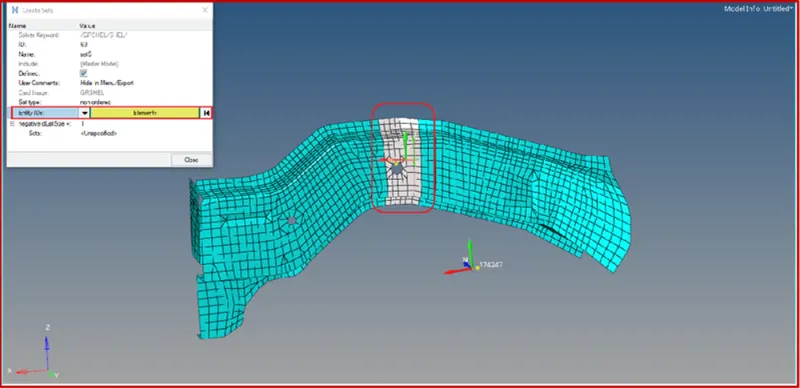
• The section is created for the two rail components which is shown in below fig.

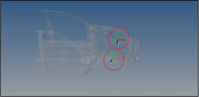
• Similarly create the sections for two shotguns,bumper,A pillar which is shown in below fig.

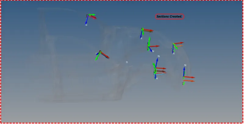
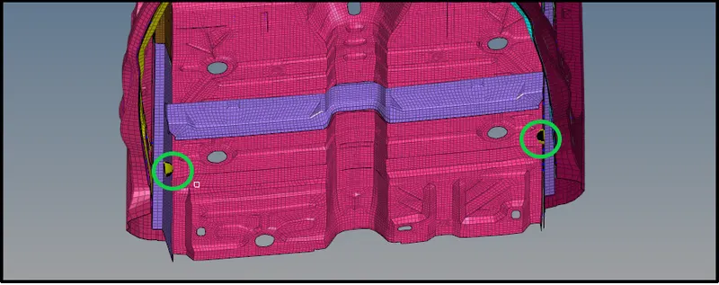
Phase 6- Create accelerometer at the B-pillar:

• Here we have to create a accelerometer at the B- pillar.To create a accelerometer,right click on the solver browser>>accelerometer>>ACCE.

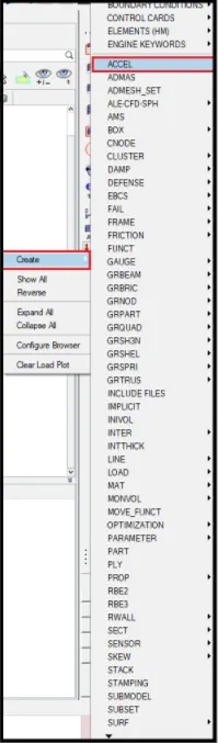
• The accelerometer is created which is shown in below fig.

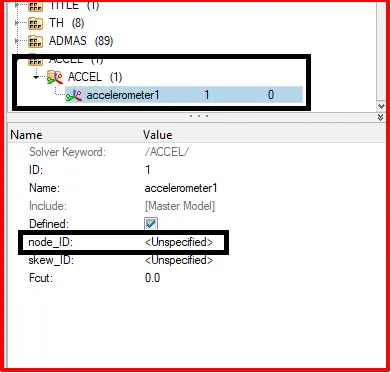
• After creating accelerometer,in the accelerometer parameter window,we have to specify the node ID.
• To specify the node ID, first we have to create a node on the B-pillar base component which is shown in below fig.

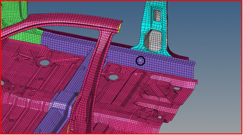
• Now create a base node to reflect that node to the other side.
• To create a base node.go to geometry>>node>>interpolate node>>select the nodes list>>no of nodes between=1>>create. which is shown in below fig.

• The base node is created,which is shown in below fig.

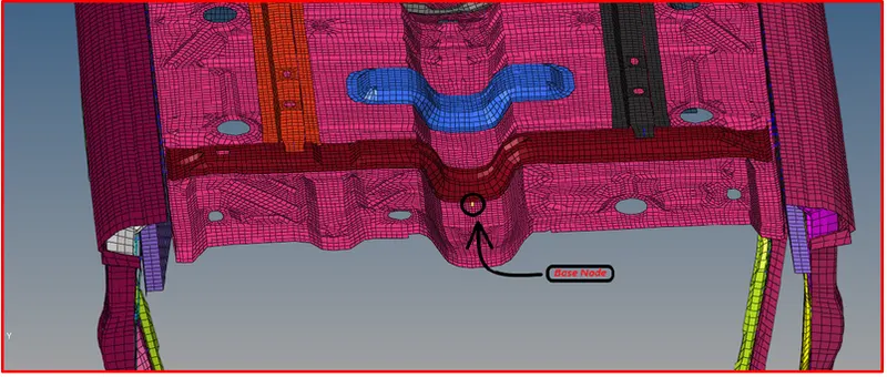
• To reflect, go to tools>>reflect,which is shown in below fig.

• The node reflected is shown in below fig.

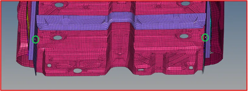
• Now select these two nodes which is shwon in above fig,to create a accelerometer for the B-pillar base component.
• The accelerometer is created for the B-pillar base component which is shown in below fig.

Phase 7- Give the initial velocity 35mph:

• Here the initial velocity should be given,cause the car should go and hit the rigid wall,so the initial vrlocity should be given.
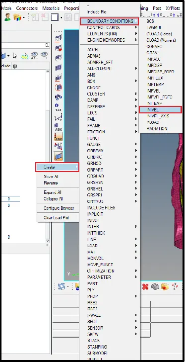
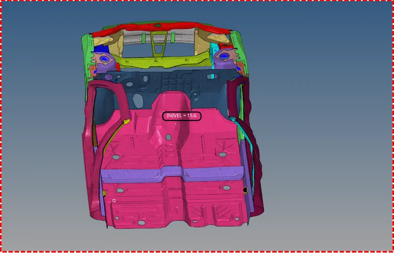
• The give initial velocity,create INIVEL Control card,to create right click on the solver browser>>create>>boundary conditions>>INIVEL.Which is shown in below fig.

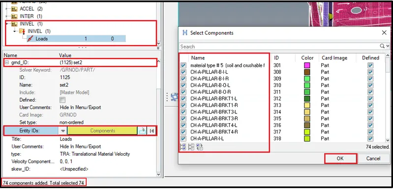
• After creating the INIVEL Card,selct all the components of the car,cause the initial velocity should be given to the whole car acuse the whole car should go and hit the rigid wall.
• Expand the gmd_ID in the parameter window and select all the components which is shown in below fig.

• According to FMVSS[{Federal motor vehicle safety standards}. Assign a inital velocity of 35mph,1mph=0.44704m/s,=35x0.4470=15.6464m/s.
• After giving the initial velocity,the model will appear as which is shown in below fig.

Phase 8- Create Intrusions on the dash wall:

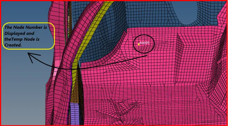
• Here we have to create intrusions at the specified nodes.
• Fiest we have to create temp node at specified location.
• To create nodes,go to display panel>>switch on the display number>>select the nodes by ID>> On,which is shown in below fig.

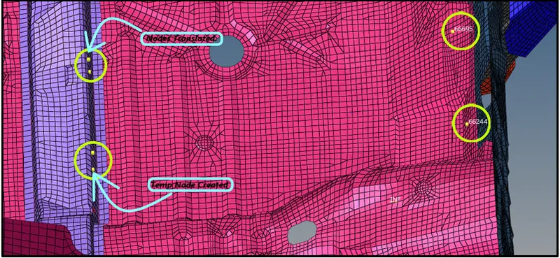
• Now translate and create the two temp nodes to the cross member components face which is shown in below fig.

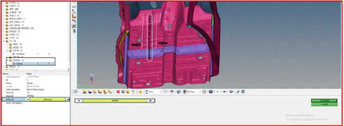
• Now create a spring,to create element,go to 1D>>spring>>select node 1 and node 2,which is shown in below fig.

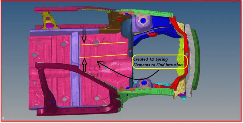
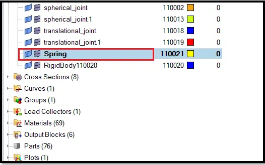
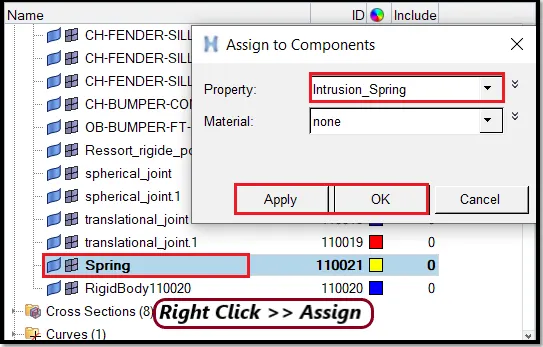
• Create a property and assign the property to the spring,collector which is shown in below fig.

Phase 9-Create rigid wall with friction 0.1:

• Rigid wall allows the user an easy way to define an interface between a rigid surface and nodes of a deformable body.
• A rigid wall is non-yielding retaining wall which is defined by the user master node and group of slave nodes.
• Rigid walls allow for an easy way to define an interface between a rigid wall surface and node of a deformable body.
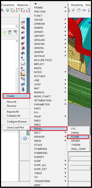
• To create rigid wall,go to solver browser right clivk>>create>>RWALL>>Plane,which is shown in below fig.

• Next the nodes should be selected to create a plane to define the rigid wall which is shwon in below fig.

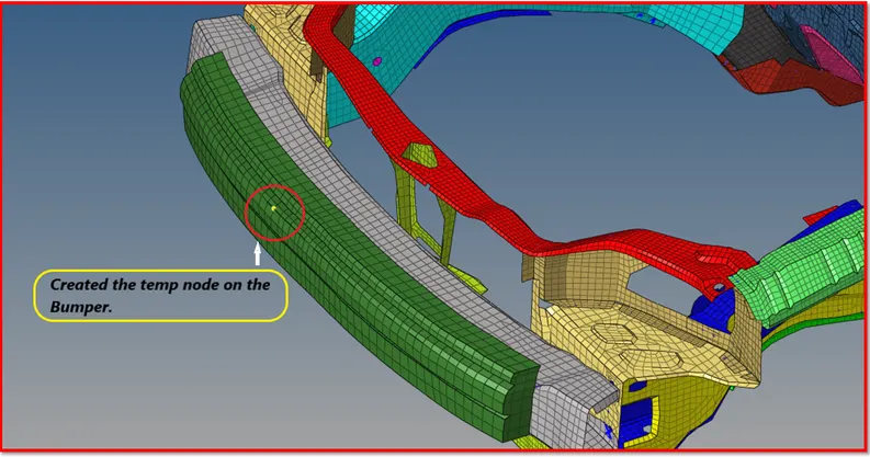
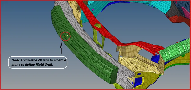
• Next translate the node to 20mm,while translating the node make it as duplicate and translate it in X-axis,which is shown in below fig.

• The node translated in X-axis to 20mm which is shown in below fig.

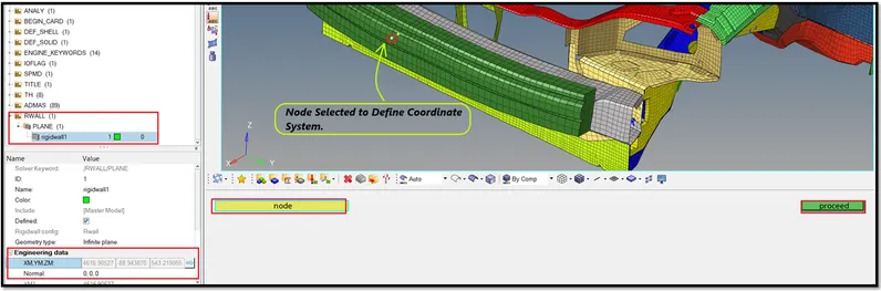
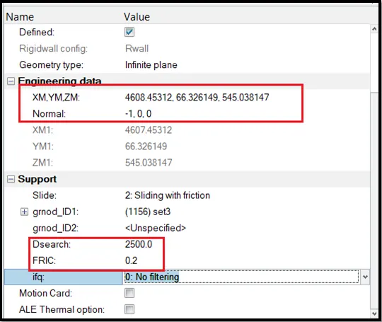
• Now select the node on the bumper to define the coordinate of the temp node [XM,YM,ZM]
• Enter the direction of the Normal [-1,0,0]
• The node selected to define coordinate system is shown in below fig.

• The D- search distance can be used around the range of 2500mm,all the nodes within the distance will be considered as slave nodes for the contact between the car and the rigid wall.

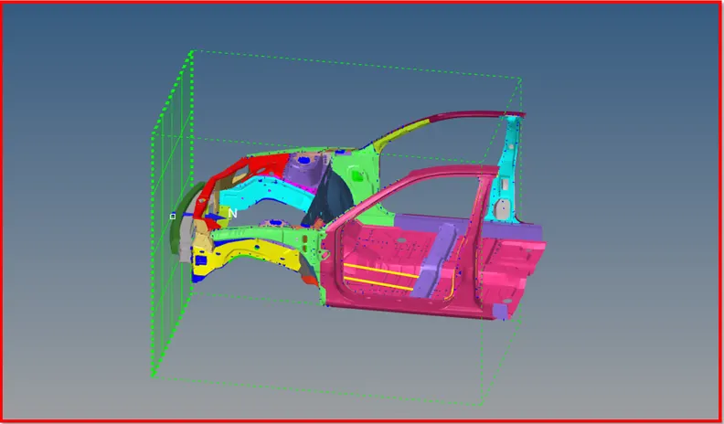
• The rigid wall is created which is shown in below fig.

Phase 10- Request TH file for the required outputs and give time step value:

• Here the timestep should be assigned to the model to run the simulation.
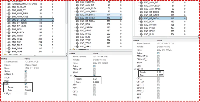
• The required values to be entered in the ENG_DT_BRICK,ENG_DT_INTER,ENG_DT_NODA Control cards which is shown in below fig.

• Next the TH ahould be requested for the Accelerometer,interfaces,sections,intrusions.

TH for Accelerometer-

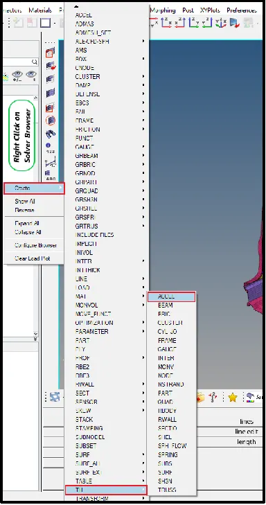
• First request TH for the accelerometer,to request TH for the accelerometer,right click on the solver browser>>create TH>>ACCEL,Which is shown in below fig.

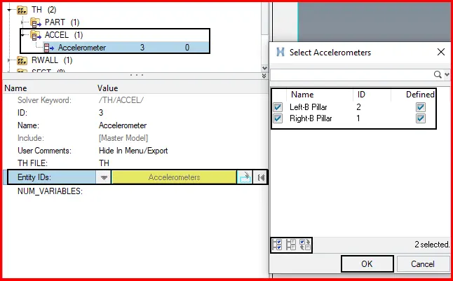
• Next at the bottom,there will be a window,there go to the entity IDs option and select the accelerometers, a window will pop up,select all and hit on ok,which is shown in below fig.

TH for interface:

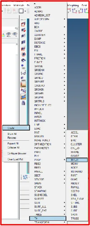
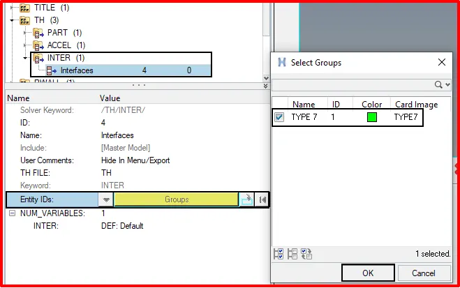
• Second request TH for the interface,to request TH for interface,right click on the solver browser>>create>>TH>>INTER,which is shown in below fig.

• Next at the bottom,there will be a window,there go to the entity IDs option and select the group A window will pop up,select all and hit on ok,which is shown in below fig.

TH for the sections:

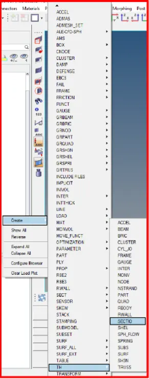
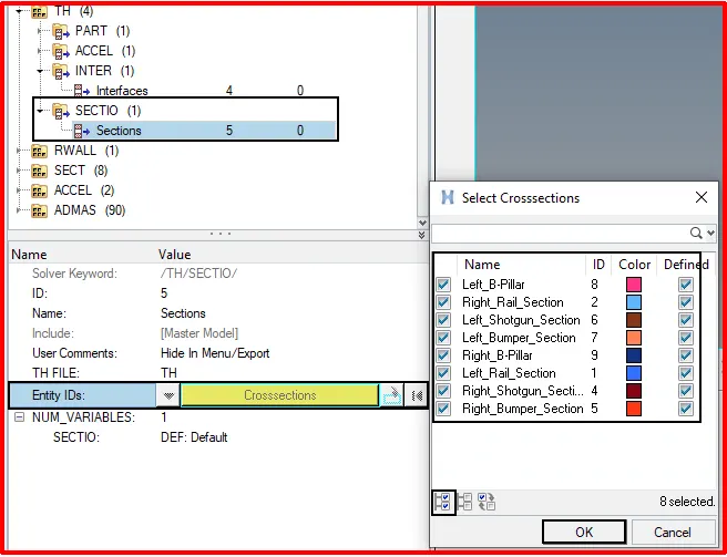
• Similarly create the TH for sections as created for previous case,which is shown in below fig.

TH for the intrusions(spring)

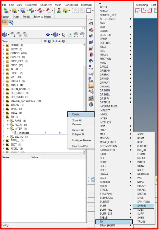
• Similarly create the TH for spring as created for previous case,which is shown in below fig

Phase 11- Run the simulation:

• Now run the simulation,to run the simulation,go to analysis panel as shown in below fig.
• Go to analysis panel>>radioss>>select the input file>>save it in different folder and rename it as test-1>>run.
• Check the include connectors,if there are any connectors in the model,the connectors will also be taken into account.
• Type -NT4 in options tab,this will make simulation faster.
• Where NT indicates no of threads,4 indicates assigning the task to 4-cores in the system.

• After completing the simulation,the radioss will pop up a solver window stating radioss job completed which indicates the simulaion has been completed.
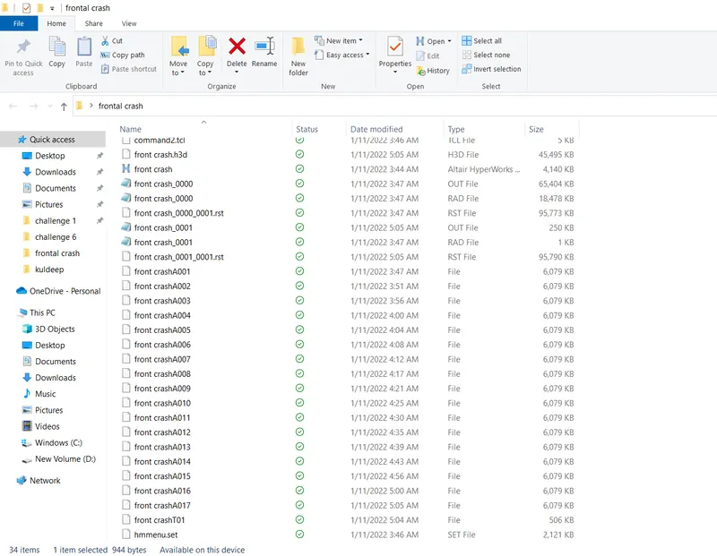
• Here the number of animation steps obtained are shown in below fig.

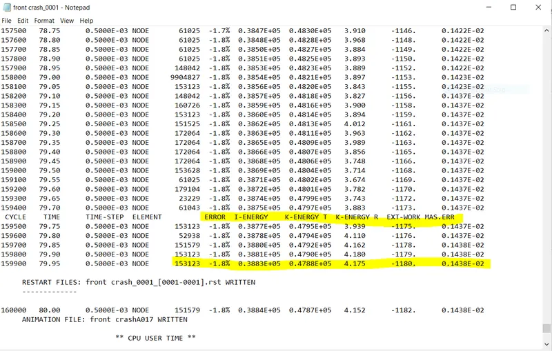
• Now go and open the 0000.1 out file with notepad.
• The obtained values for Energy error,mass error,internal energy error,kinetic energy error and contact energy error has been shown in below fig.

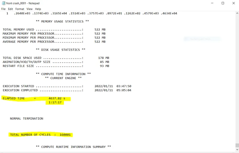
• The time taken to complete the simulation and the elapsed time is shown in below fig.

Phase 12-Post Processing:

• 1) Review the simulation using-Hyperview
• 2) Plot the graph using-Hypergraph 2D

• 1) Review the simulation using hyperview:
• Hyperview allows for loading and viewing result files obtained from several sources.
• Based on the solver type of the files and results you would like to visualize and analyze,there are different ways to load the input deck and their corresponding results into hyperview.
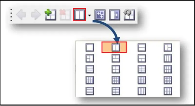
• First to begin the postprocessing in the hypermesh,split the screen as shown in below fig.
• Importing the animation file.h3d into the hyperview.

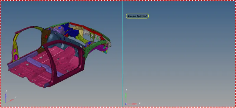
• And then activate the client hyperview.

• To access the load model panel
• Select load model button from the hyperview panel and open.h3d file as shown in below fig.

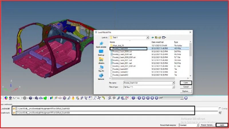
• After loading the model into hyperview,it will be represented as shown in below fig.
• After importing the .h3d file into the GUI,enable the contour.
• The contour tool create contour plots of a model graphically visualize the analysis results.
• To enable contour,go to results toolbar>>contour.

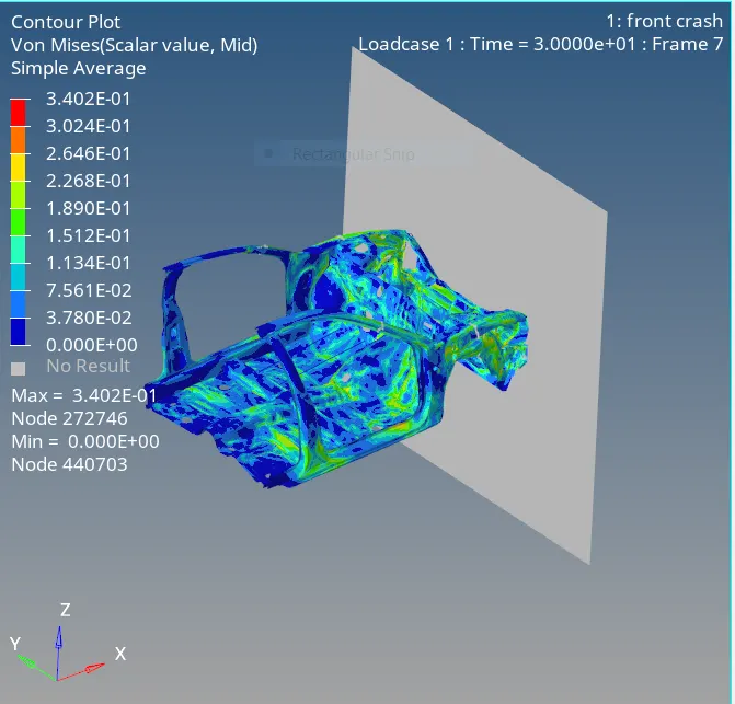
• Now switch to the Von misses stress in result type and select the component,select the averaging method as simple and then click apply as shown in below fig.

• After applying,run the simulation,the simulation animation in terms of von misses stress and displacement is shown in below fig.

Check for the Intrusions:

• After running the simulation,we have to check for the intrusions.
• Note: The allowbale intrusion is 15 cm.
• To check for the intrusion,measure the distance between the springs where we created.
• To measure,go to measure tool from hyperview and select the end node of the spring to know the distance between them,which is shown in below fig.

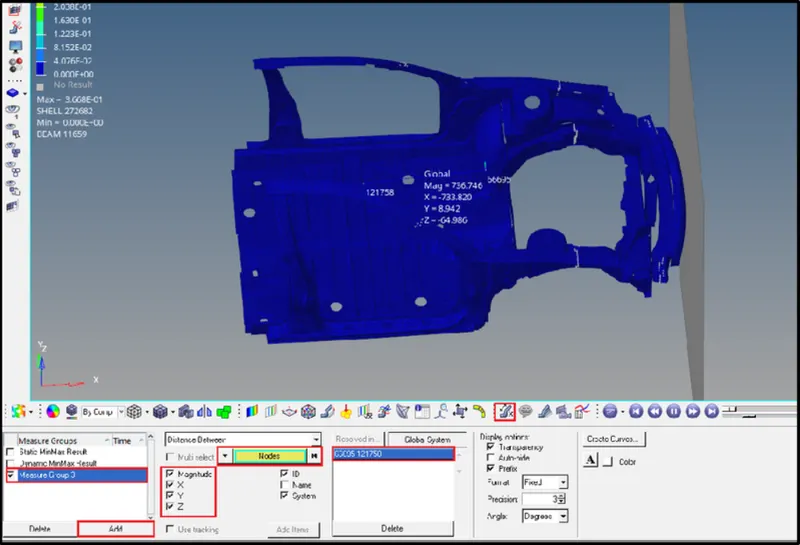
• After defining the nodes at the end of the spring at the initial position before the collision.The magnitude for the spring at the node 66244 is 736.746mm.
• After defining the nodes at the end of the spring after the collision,the magnitude for the spring at the node 66244 is 644.678 mm.

Intrusion Results:

1) spring [At node 66244]= 736.746-644.678= 9.1966 cm.
2) spring [At Node 66695]= 759.192-626.617= 132.575=13.2575cm.

2) Plot the graph using-hypergraph 2D:

• Now plot the graph using hypergraph 2D,we are plotting the graphs to see what is happening in the rail component.
• Hypergraph 2D is powerful data analysis and plotting tool with interfaces to many popular file formats.
• It is sophiscated math engine capable of processing even the most complex mathematical expressions.
• Hypergraph 2D combines these features with high quality presentation output and customization capablities to create a complete data analysis system for any organization.

• Here switch to the hypergraph 2D to the plot the graphs.
• To switch,go to client selector>> choose the hypergraph 2D as shown in above fig.
• [Note: Before plotting the graphs,make sure to split the screen into three or four then plot the graphs.
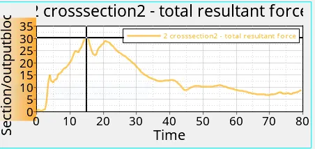
• The first graph is plotted for the right rail at the created section.
• To plot the graph,go to hypergraph 2D>>Data file>> frontal_crashT01>>Apply.

Right Rail:

• The graph obtained for the right rail which is shown in below fig.
• The maximum sectional force on the right rail is 30.535 KN

Left Rail:

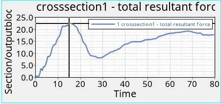
• The graph obtained for the left rail rail which is shown in below fig.
• The maximum sectional force on the Left rail is 22.578 KN.

Right shotgun:

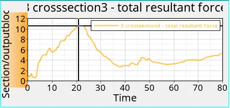
• The graph obtained for the right shotgun which is shown in below fig.
• The maximum sectional force on the right shotgun is 10.661 KN.

Left shotgun:

• The graph obtained for the left shotgun which is shown in below fig.
• The maximum sectional force on the left shotgun is 11.619 KN

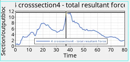
Right Bumper:

• The graph obtained for the right bumper which is shown in below fig.
• The maximum sectional force on the right bumper is 12.6944.

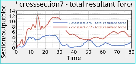
Left Bumper:

• The graph obtained for the right bumper which is shown in below fig
• The maximum sectional force on the left bumper is 15.183 KN.

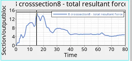
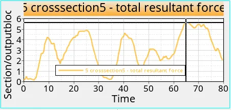
Right B-Pillar:

• The graph obtained for the right B- pillar which is shown in below fig.
• The maximum sectional force on the right B-Pillar is 4.846 KN.

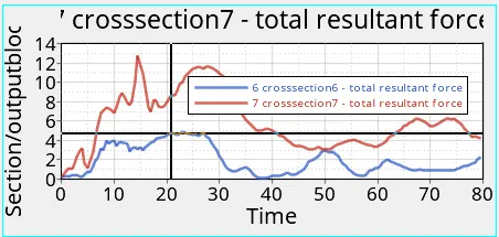
Left B-Pillar:

• The graph obtained for the left B-pillar which is shown in below fig.
• The maximum sectional force on the Left B-Pillar is 5.634 KN.

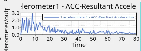
Right B-pillar base component Acceleration:

• The graph obtained for the right B- pillar base component acceleration which is shown in below fig.
• The maximum acceleration on the right B-pillar base component is 2.962 m/s.

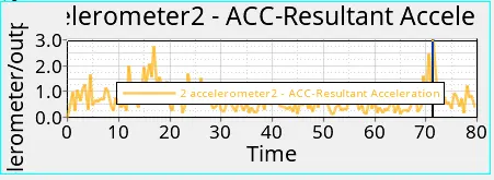
Left B- pillar base component acceleration:

• The graph obtained for the right B- pillar base component Acceleration which is shown fig.
• The maximum acceleration on the right B-pillar base component is 2.979 m/s.

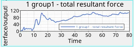
Interface [type 7 contact]:

• The graph obtained for the interface [type 7 contact is shown in below.
• The maximum force is 110.623 KN

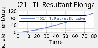
Intrusion spring with node 66244:

• The graph obtained for the intrusion spring with node 66244 is shown in below fig.
• The maximum intrusion value obtained for this node is 109.131 mm which 9.1508 cm.

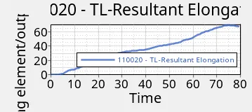
Intrusion spring with node 6695:

• The graph obtained for the intrusion spring with node 66655 is shown fig.
• The maximum intrusion value obtained for this node is 69.512 mm which 13.1625 cm.

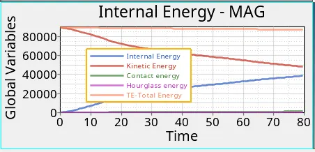
All Energies:

• All the energies have been plotted which is shown below fig.

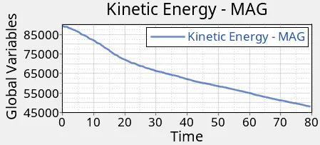
Kinetic energy:

• The kinetic energy decreases due to decrease in velocity because the given velocity which may reduce.
• The kinetic energy graph is shown in above fig.

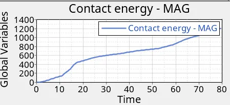
Contact Energy:

• The contact energy will increase slightly when the car hits the rigid wall because only some of the elements at the front will be having the contact.
• The contact energy graph is shown in above fig.

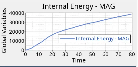
Internal energy:

• The internal energy will gradually increase.due to increase in displacement.
• The internal graph is shown in above fig.

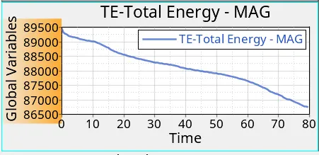
Total energy:

• The total energy will be slightly decreasing due to decrease in kinetic energy.
• The total energy graph is shown in above fig.

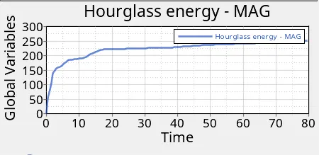
Hourglass energy:

• There will be no hourglass energy because the element formulation is specified with recommended parameters.
• The recommended parameters have been assigned,here Ishell=24 QEPH is used,due to this there is no hourglass effect.
• The hourglass energy graph is shown in fig.

Result:

• Hence the COG from the initial position has been changed to the required position by mass balancing.
• Hence the penetrations and intersections has been verified successfully.
• Hence the interfaces created newly.
• Hence the accelerometers created at the base of B-pillar to obtain the acceleration.
• Hence the initial velocity was assigned.
• Hence the springs were created to obatin the intrusions.
• Hence the rigid wall was created successfully.
• Hence the TH for all inputs were created in order to obtain outputs.
• Hence the simulation was runned successfully without any errors.
• Atlast all the graphs were plotted with the obtained results.

Conclusion and learning outcome:

• How to change the COG position.
• How to check for the penetration and intersections.
• How to create the interfaces and how to find connectivity,to check whether the free parts exsist in the components.
• How to create the accelerometers.
• How to assign the initial velocity.
• How to create the springs to obtain intrusions.
• How to create a rigid wall.
• How to request outputs.
• Learned about the FMVSS 208.
• Learned about the sectional forces,axial forces.