Assignment 6

Skill lync assignment 6

Aim: The objective is to check the given component for consistent unit system, geometric errors, rigid bodies, penetrations and other relevant parameters. The component is then to have mass added to reach a level comparable to that of the full scale model provided, while maintaining the location of the center of gravity. Other relevant boundary conditions, such as rigid wall and initial velocity are to be added, along with time step range and time frame for animation, after which the component is to be simulated in RADIOSS and checked for forces and accelerations at the specified rail cross-sections. The errors involved in the final output are to be identified and rectified.

Case study: The given component illustrates the front section of a car chassis, as shown below.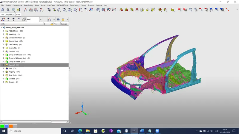

Figure 1: Car chassis model

The component has a total mass of 188.43 kg (defined with kg, mm, ms units) with the COG roughly at the gear-stick region.

The second component provided is a full scale variant of the first with included body panels, engine & powertrain components and tyres, as shown below. The total mass of this component is 1216.5 kg with the COG at rhe same area as the first component.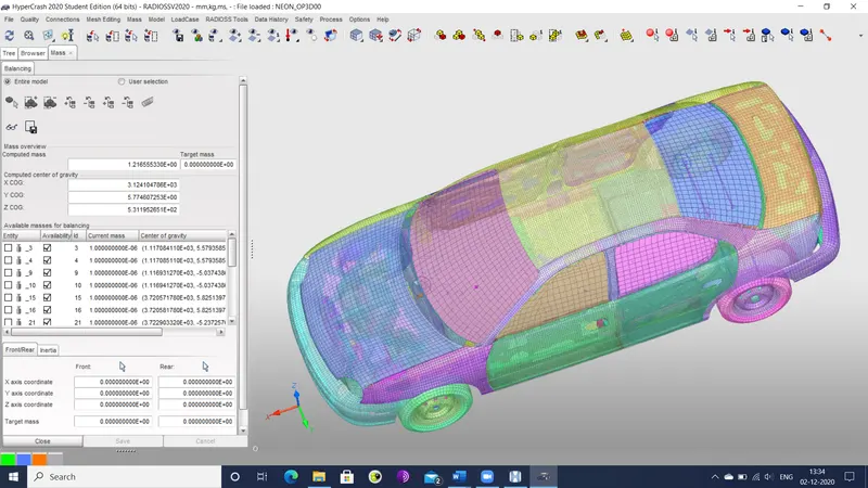

Figure 2: Full scale car model

Procedure: The given partial component is worked on and simulated through the following sequence of steps.

1. The starter file for the first component is checked for the units.
2. The first component is imported into the hyper-crash workspace.
3. The contact interfaces are replaced with a single type 7 contact and optimized for self-impact with a friction coefficient of 0.2. Intersections and penetrations are checked and rectified by the quality>check all solver contact interfaces.
4. Rigid bodies are checked using the mass>rigid bodies menu selection. The rigid bodies are checked for automatic master node generation and inclusion of said master node in time history. In addition to this, the center of gravity computation (ICOG) parameter is set to the value of 2, where the overall COG is computed using only the slave nodes of the rigid bodies.
5. A plane rigid wall is created near the front side of the component by the load case>rigid wall menu selection. The resultant wall with normal vector is shown below.

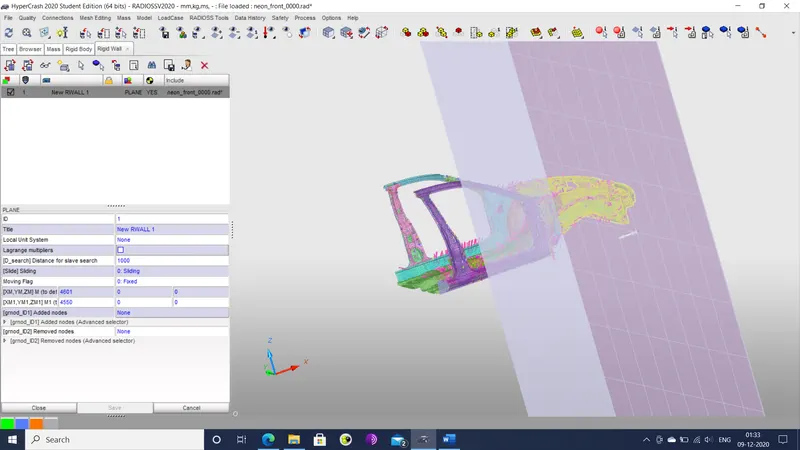
Figure 3: Rigid wall definition

6. An initial velocity is imparted to the component by the load case>initial velocity menu selection. The velocity set is in the x-direction with a magnitude of 35 mph, i.e. 15.6464 mm/msec.
7. The mass>balancing menu selection is used to see the overall mass and COG of the component. Here, it is apparent that the overall mass is 188.4254437 kg and that the COG is located at the coordinates (3163.9563, -2.667949047, 440.4097942).
8. The values of the applied masses are modified so that the COG is shifted to the region between the front seats and the overall mass crosses 700 kg. The added masses are heavily magnified to simulate seat & passenger pairs that weigh 100 kg each, a drivetrain section that weighs 240 kg and 2 sections of axial floor beams weighing 60 kg each. The final COG is located at the coordinates (2696.569788, 24.08635816, 327.3459192). The screenshot is shown below.

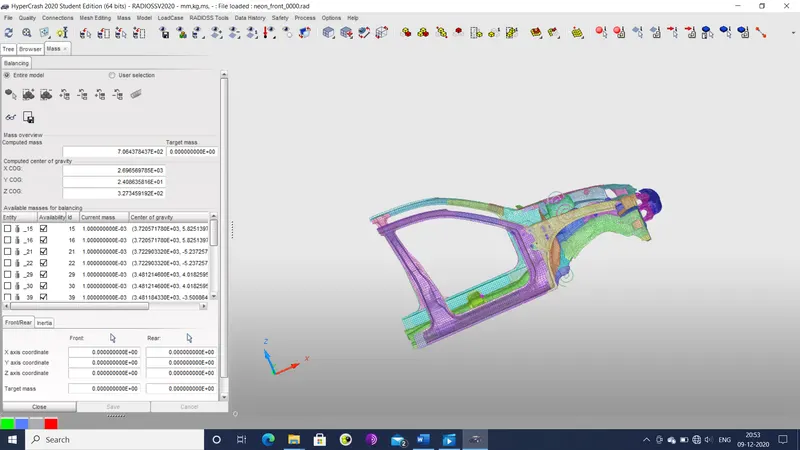
Figure 4: Final mass and COG

9. In the browser tree, the control card for RUN is checked for overall time frame and it is ensured that the run time is 80 msec.
10. The control card for DT_ELTYPE_KEYWORD_IFLAG is modified so that minimum time step for all element types is 0.1 microsec or 0.0001 msec, time step scale factor is 0.67 and time step control type is CST.
11. In the property section of the browser tree, the solid element formulation is changed to HEPH, while shell element formulation is changed to QEPH.
12. The data history>section>section menu selection is used to generate sections where axial forces are to be measured. 3 nodes are selected for the section plane and unnecessary elements are removed from the section. The section for the A-pillar is shown below.

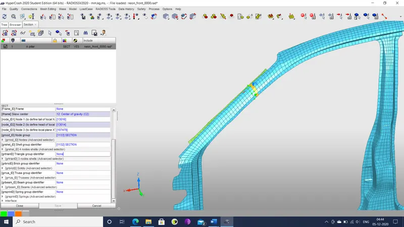
Figure 5: A pillar section definition

13. Similar sections are generated at the shotgun region and at the node with ID 174247.
14. Accelerometer nodes are placed at the base of the B-pillars using the data history>accelerometer>accelerometer menu selection. Their locations are illustrated below.

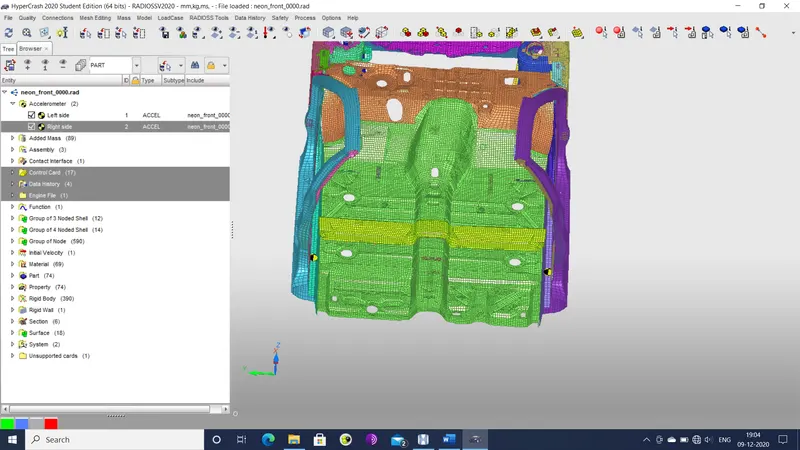
Figure 6: B pillar accelerometers

15. For measuring the intrusions at nodes 66695 and 66244, A local coordinate system is generated in the form of a skew at a point on the component that is not expected to deform in any considerable amount. This is done by the RADIOSS tools>skew/frame menu selection. The origin of this skew is shown in the image below.

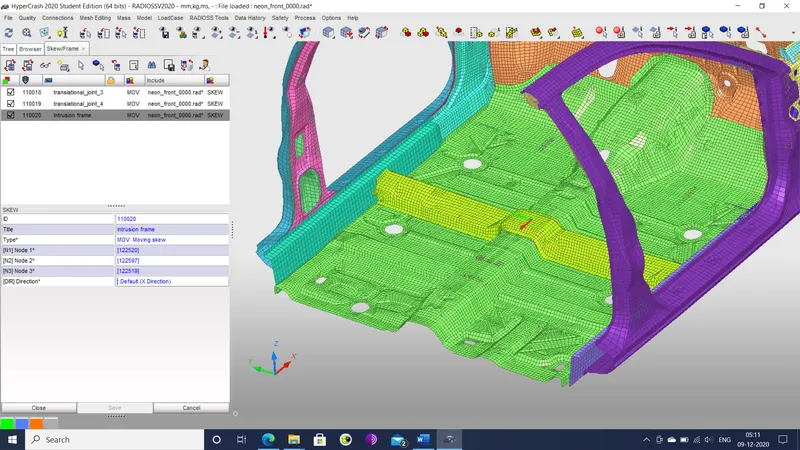
Figure 7: Skew definition

16. The data history>time history menu selection is used to bring up the time history options, where the output files for time history plots are selected. In the TH SECTIO section, the variable being computed is changed to normal force (FN) so that normal force at the defined sections is plotted.
17. A new TH NODE section is defined for measuring the intrusion at the relevant nodes. The individual nodes are defined and the skew defined earlier is used as the frame of reference and the displacement in the x-direction (DX) is set as the measured variable. The result is shown below.

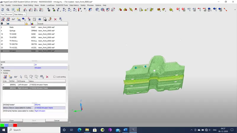
Figure 8: Node definition for intrusion nodes

18. Another TH NODE section is generated for measuring the axial forces on the rails from the bumper. The variable to be measured is the reaction force in the x-direction (REACX). The selection is shown below.

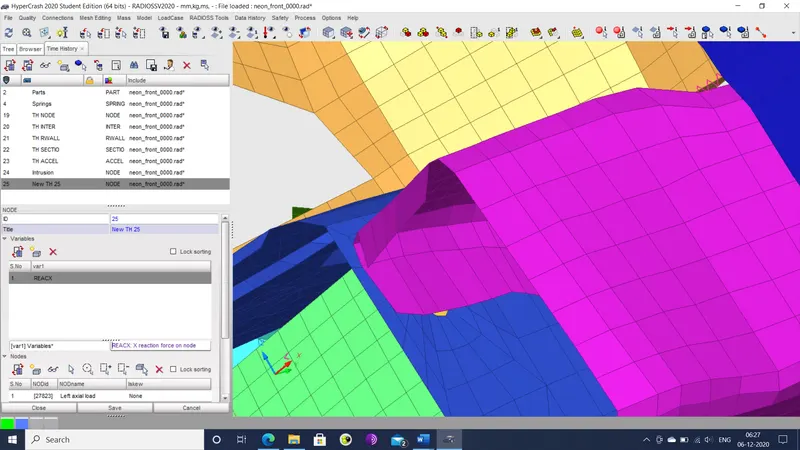
Figure 9: Node definition for reaction force measurement at bumper

19. The unnecessary time history plots are deleted from the component.
20. The model quality is checked with the quality>model checker menu selection and any errors that pop up are rectified. One of the errors that require manual correction are the presence of existing, poorly defined skews for translational springs for the suspension. These skews are deleted after being deemed unnecessary.
21. The output files are finally exported and run in the RADIOSS solver. The output plots and animations are loaded into hypergraph 2D and hyperview respectively and analysed.

Results: The following were the results of the simulation.

• The overall simulation time was 3 hours, 35 minutes and 13.88 seconds, while the total number of cycles was 440493. This was the reduced amount of computation time that could be achieved after adjusting rigid body parameters such that COG computation (ICOG) was done only by the slave nodes. This time may have potentially been reduced even further if COG computation was set to use only master nodes, while sacrificing accuracy of results.
• The following is the time history of the plot of the various types of energies.

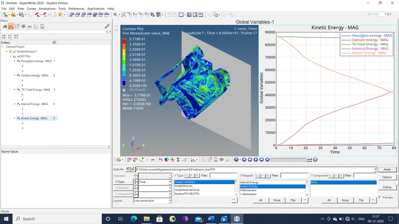
Figure 10: Energy plot

The hourglass energy is practically non-existent in the component. Total energy is relatively constant throughout the simulation, which verifies the absence of any significant hourglass energy. There is a slight but steady increase in contact energy. This contact energy is about as low as it can be due to the minimum activation gap being set to the lowest possible value of 0.5 mm. Overall, the contact energy is far less than the internal and kinetic energies. Thus, the increase in internal energy is roughly equal to the drop in kinetic energy.

• The plot of the time step is shown below.

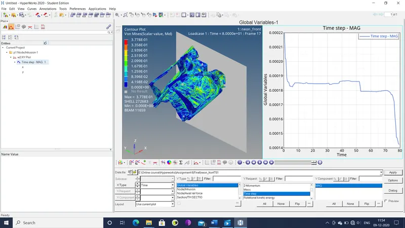
Figure 11: Time step plot

The time steps remain within the range of 0.1 – 0.5 microseconds. However, towards the end of the simulation, there was a significant drop in the same. Had the run time been longer, the time step would have dropped enough to activate the time step correction algorithm.

• The intrusions at the driver side foot board are plotted as shown below.

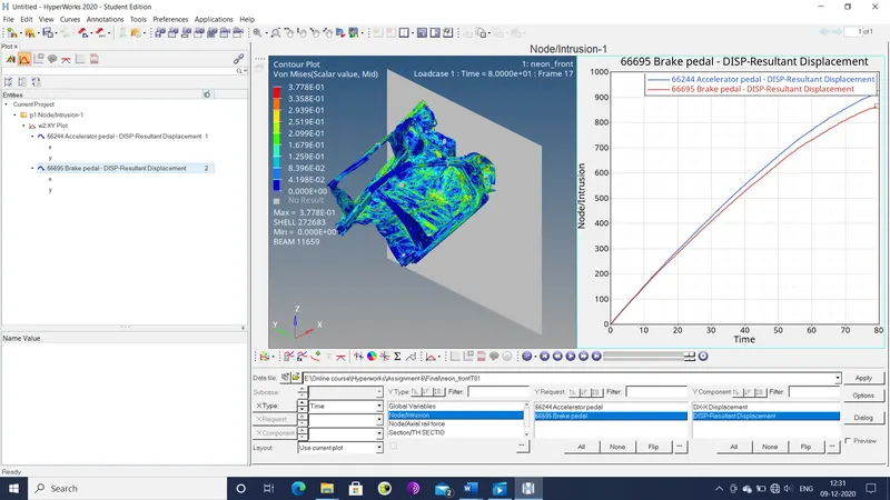
Figure 12: Intrusion plot

The intrusion is shown to reach nearly a metre. However, this may not be an entirely accurate value since the region where the reference skew was defined deforms noticably.

• The cross-sectional forces in the component are plotted below.

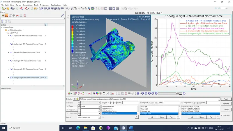
Figure 13: Cross-sectional forces plot

Here, the greatest amount of force is experienced in the inner rail sections. The peak amount of force experienced here is about 33 kg*mm/msec², i.e. 33 KN.

• The axial forces at the bumper did not register at all. So the method used to determine it (reaction force at node) turned out to be ineffective.
• The accelerations at the specified locations are plotted below.

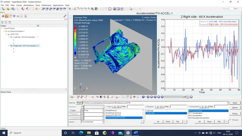
Figure 14: Acceleration plot

The acceleration in the x direction reaches upto roughly 0.1 mm/msec² or 100 m/sec². This is about the type of acceleration to be expected in a crash. These values are not identical for both sides though. This could be due to the geometry of the component, as it is not strictly symmetric. In addition to this, the COG of the component is also not precisely at the middle of the component, which causes the subtle difference in acceleration on either side. The acceleration is also shown to fluctuate wildly, especially in the left B pillar. This indicates a possibly unrealistic amount of vibration in the component. This could potentially be solved by altering the gap scale correction factor for the type 7 contact used, so that contact forces are less likely to arise and generate these vibrations.

• The animation itself shows a rather unusual buckling of the component. Here, the component tends to buckle upwards, particularly at the front suspension. This is due to the springs that were left in the respective area.
• The 0001.out file verifies that time step fell within the acceptable range. As a result, the time step correction algorithms were not activated and there was no mass error in the entire animation. Also, the hourglass energy error drops until it reaches a minimum value of -2.1%, which is an acceptable value.

Conclusion: The component given was suitably pre-processed, simulated and post-processed. The discrepancies in the output plots were identified and possible remedies were explored.