Assignment 5-RADIOSS Interfaces & Study of Effect of Notches Challenge
Assignment 5-RADIOSS Interfaces & Study of Effect of Notches Challenge
1. Aim
- For the given model, perform meshing using the specified target element length.
- Run the crash tube simulation for the mentioned cases
- Plot appropriate graphs. Compare and analyse the results of each case.
2. Objective
For Meshing
- Using hypermesh, Import, clean and mesh the model using specified target element length and quality criteria.
- Using 1D connectors for the proper connection between the components
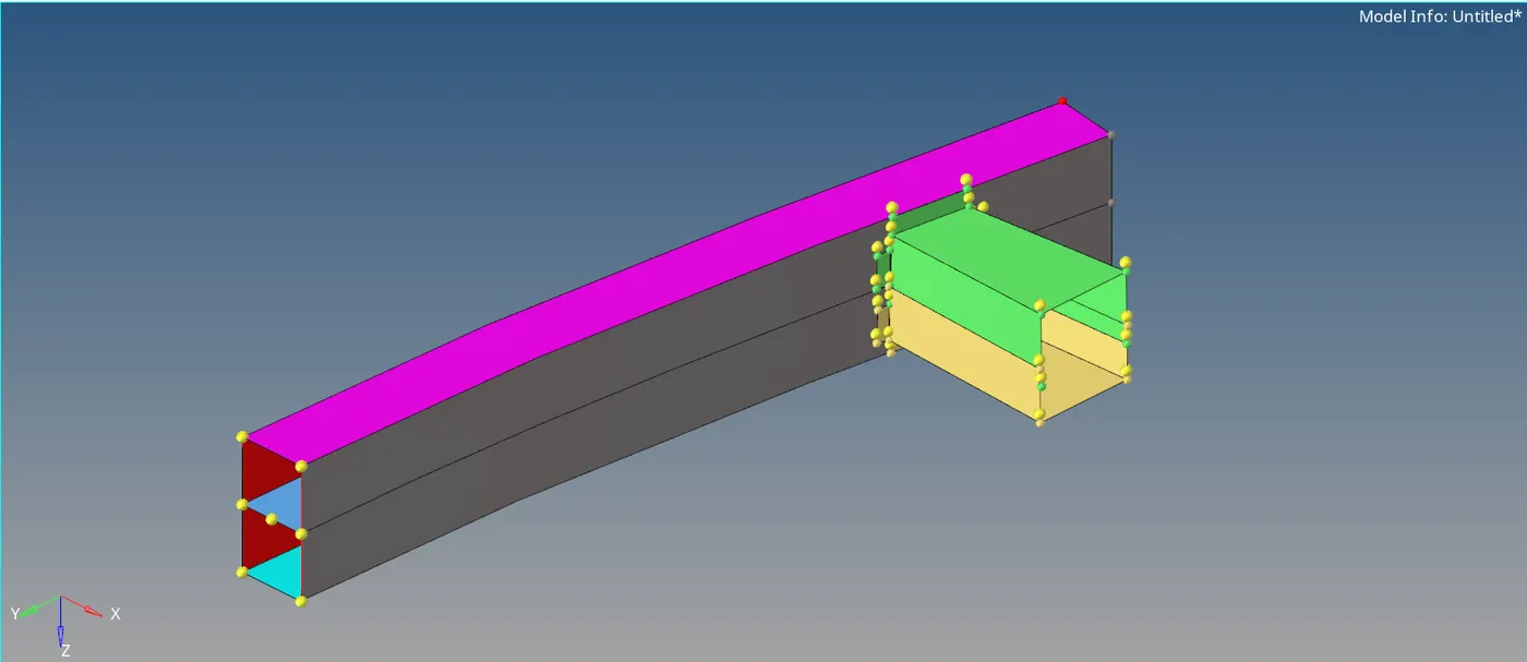
Fig 1: Isometric View Of Bumber Model
For Crash Tube Simulation
- Using hyper mesh, Import the crash tube file and simulate the following cases
Case 1: Run the crash tube model as it is.
Case 2: Change the Inacti=6 and run.
Case 3: Create the type 11 contact and run.
Case 4: Remove both notches and remove boundary condition on rigid body node then run.
Case 5: Create a new notch in the middle, select the whole section and run.
Case 6: Create a new notch with nodes only from opposing 2 faces and run.
- Plot RWALL forces, contact forces, and internal energy Create TH/PART for all parts and compare results for all cases. Analyse the change in internal energies and the effect of notches.
- Plot energies and note the differences.
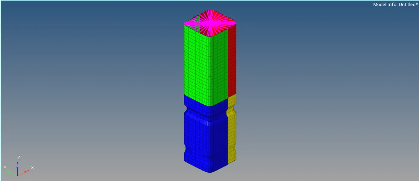
Fig 2: Isometric View Of Crush Tube Model
3. Procedure
- For Meshing
Step 1: Importing and Geometry Cleanup of the Model
Import the model to the hyper mesh. Switch to topo mode and correct all the errors present in the geometry using the appropriate tools.
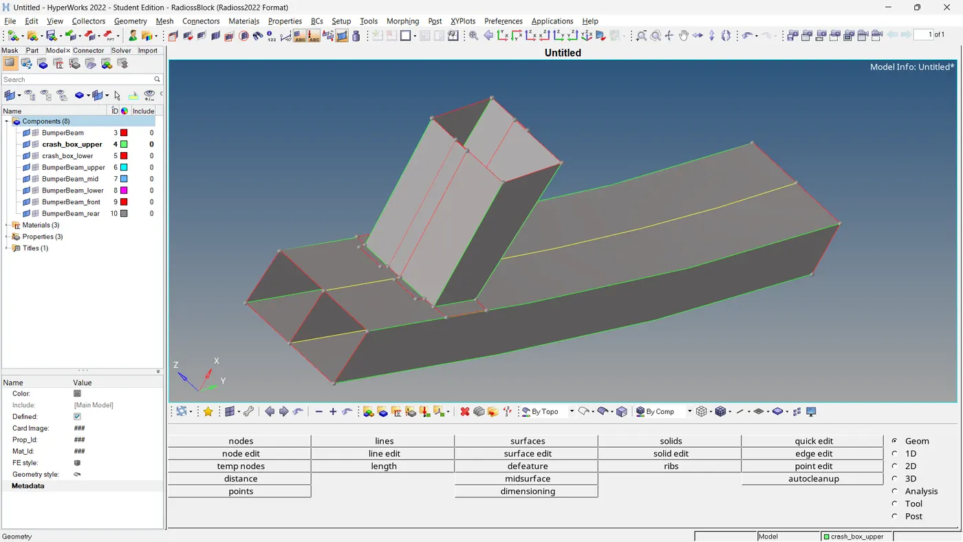
Fig 3: Geometric Cleanup of The Model
Step 2: Adding Target Element Length and Meshing
After the geometric cleaning, Using automesh mesh the surface with a target element length of 6 units. Adjust the number of nodes to avoid the formation of trias.
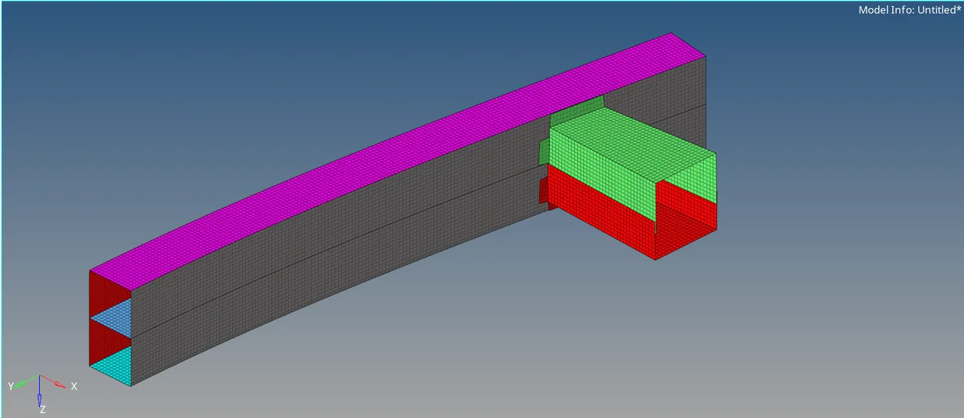
Fig 4: Meshing Of Components
Step 3: Creating 1D Elements
We have to connect the crash boxes and bumper beams, as well as the 2 sides of the crash boxes to each other. For creating connectors, we use 1D elements.
- 1D >> Connectors
Here we use seam connectors. The Seam connectors are created by
- Seam >> Seam >> Location =Nodelist From Target Component, where need the connection. >> Spacing= 6 (Target Element Length) >> Connect What= Select Both Components >> Type= Weld >> Property = Create A Property and Select >> Tolerance =10 >> Create.
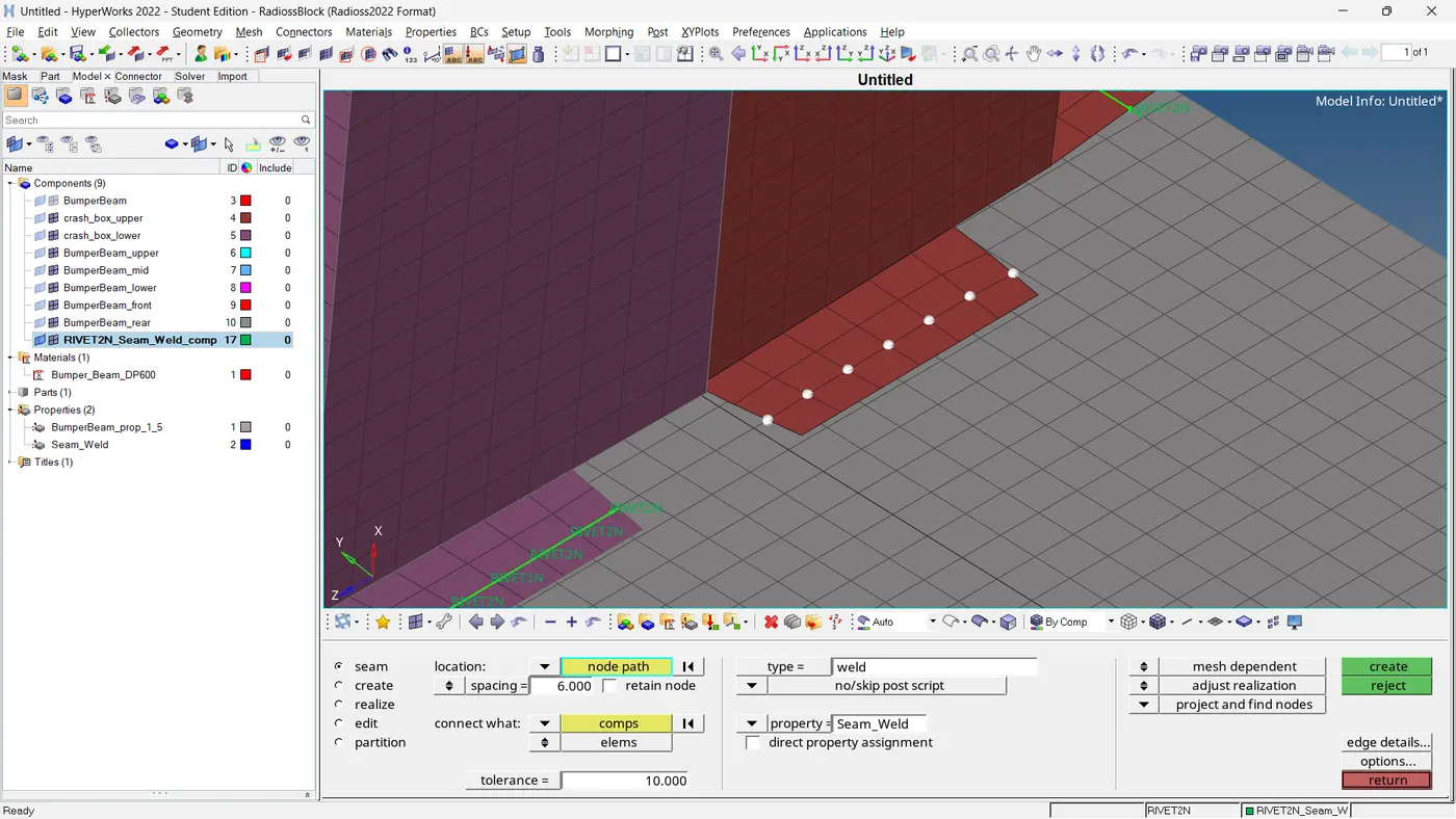
Fig 5: Creating 1D Elements
We can use the element type as per the specifications mentioned in the cases. Because we use RADIOSS as a profile, it has fewer element types than Opistruct.
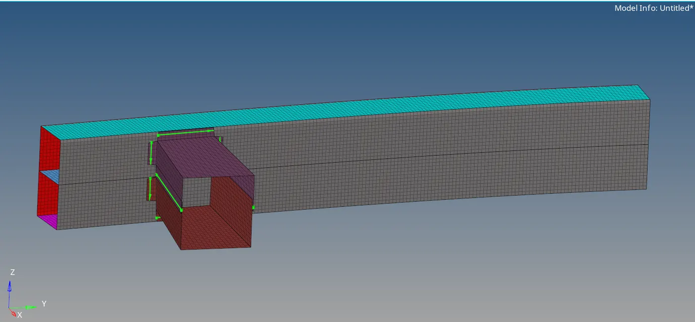
Fig 6: Final Result (Objective 1)
2. For Crash Tube Simulation
Step 1: Importing and opening the Model in Hyper Mesh RADIOSS
Initially, the beam file 'Crush_tube_0000.rad' is imported to hyper mesh through the solver deck.
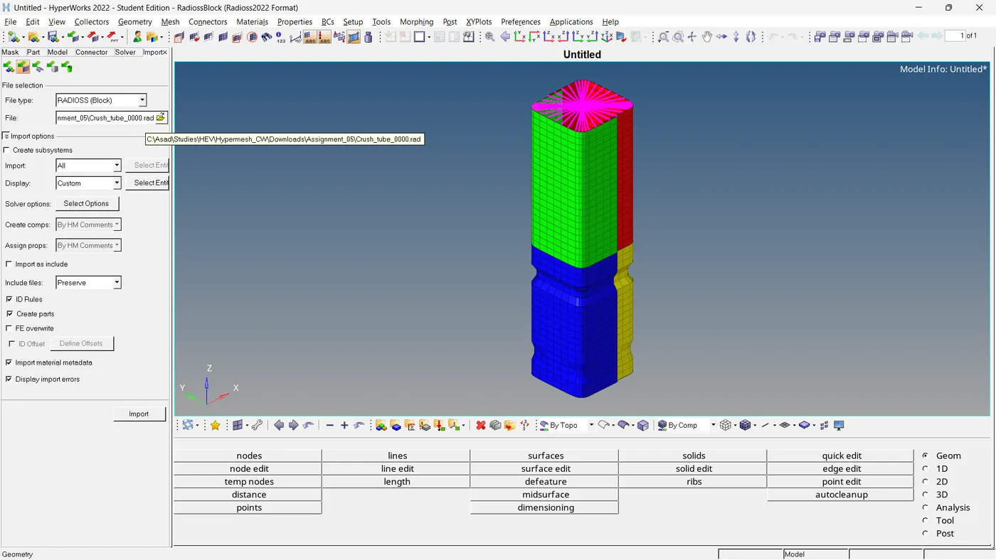
Fig 7: Importing Of Model
For our better understanding of the positions of all our components rename the components. Then we have to create Time History (TH) for all parts and it helps to plot graphs and compare the results in each case.
- Model Browser >> Right Click >> Output Block >> Rename 'TH_Part_All' >> Entity IDs = Components >> Assign All Components.
The thickness of each component is
- 2mm- Top_PSHELL_01 / Top_PSHELL_02
- 3mm- Bottom_PSHELL_01 / Bottom_PSHELL_02
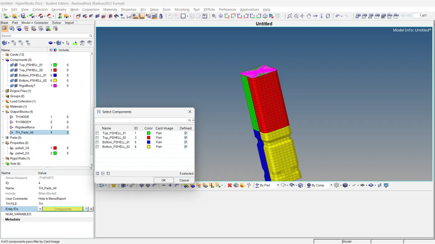
Fig 8: Output Block Creation
Case 1: Run the crash tube model as it is.
Step 1: Setup Case Definitions
As per case 1, we have to simulate the model as it is. There are no changes to the values. Import 'Crushtube_0000.rad' to hyper mesh using the solver deck.
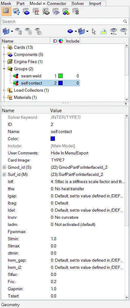
Fig 8: Interface Type and Its Values
From here, we can understand that the assigned interface is Type 7. Type 7 interface simulates all types of impact between a slave node and master segment. Respective values defined for type 7 are
| Sl No. | Parameter | Values |
| 1 | Istiff | 4 |
| 2 | Igap | 0 |
| 3 | Gapmin | 1.0 |
| 4 | Iform | 2 |
| 5 | Iacti | 0 |
| 6 | Stmin | 1 |
Table 1: Type 7 Parameters and Their Values
Step 2: Simulate the Model and Analysis of the Results. Save the filename as 'CrushTube_NoChanges_Case1_0000.rad'
The simulation is done by following,
- Analysis >> Radioss >> Browse Input File Location >> Option = -nt 4 (No. Of Threads) >> Radioss
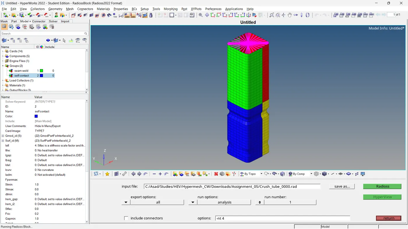
Fig 9: Loading Simulation Using Hyper Mesh (Case 1)
After the simulation, a job summary will pop up and it gives whether the simulation is completed or not. After a successful simulation, we can inspect the animations (.h3d file) through the hyper view. Check the errors from the output file, if it is in between the acceptable range, we can proceed with the simulation.
- Energy Error = -3.8%
- Mass Error = 0.0%
The errors are within the acceptable range. So we can continue with the model. Using the hyper view, we can make the contours with Von Mises Stress.
- Contours >> Result Type = Von Mises (S) >> Averaging Method = Simple >> Apply
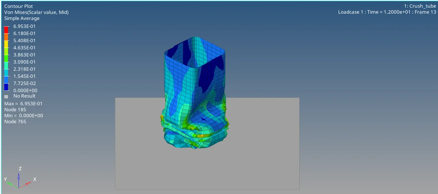
Fig 10: Contours- Von Mises Stress (Case 1)
Step 3: Plotting Necessary Graphs Using Hyper Graph 2D
The plots are drawn using the hypergraph 2D, by opening the Time History File of the model and it can be used for the comparison between other cases. Plot time history of
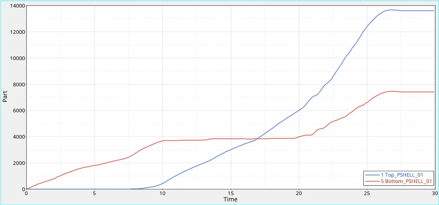
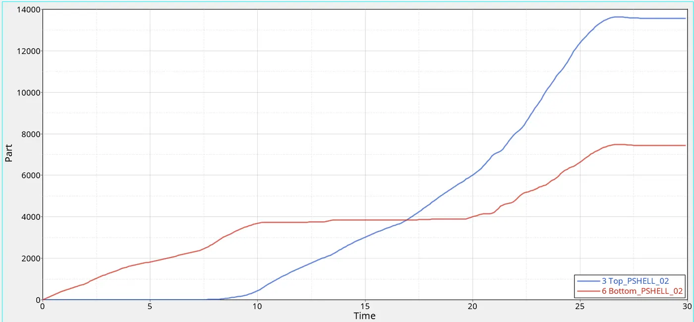
Plot 1,2: Time Vs Internal Energies (Case 1)
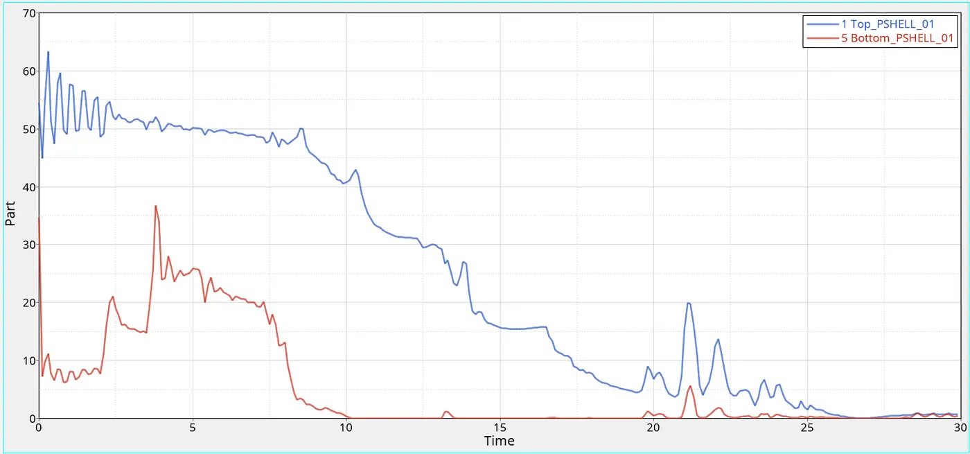
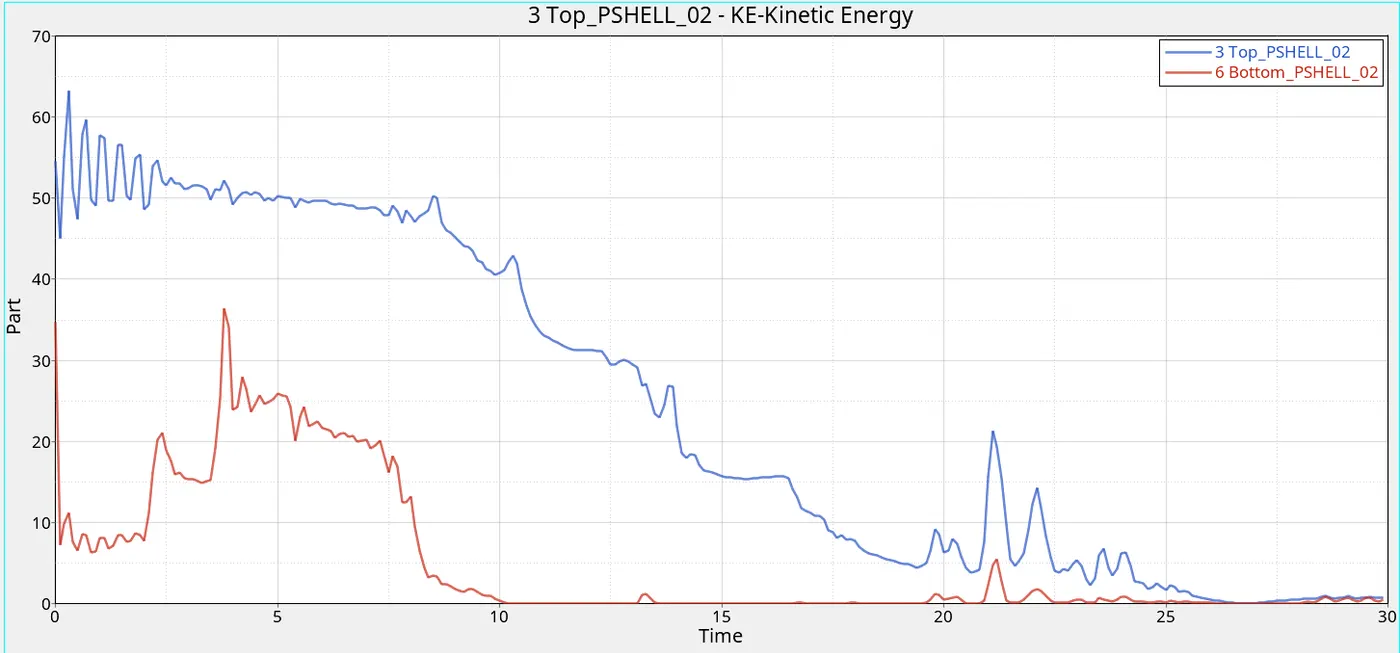
Plot 3,4: Time Vs Kinetic Energies (Case 1)
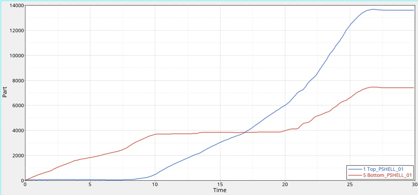
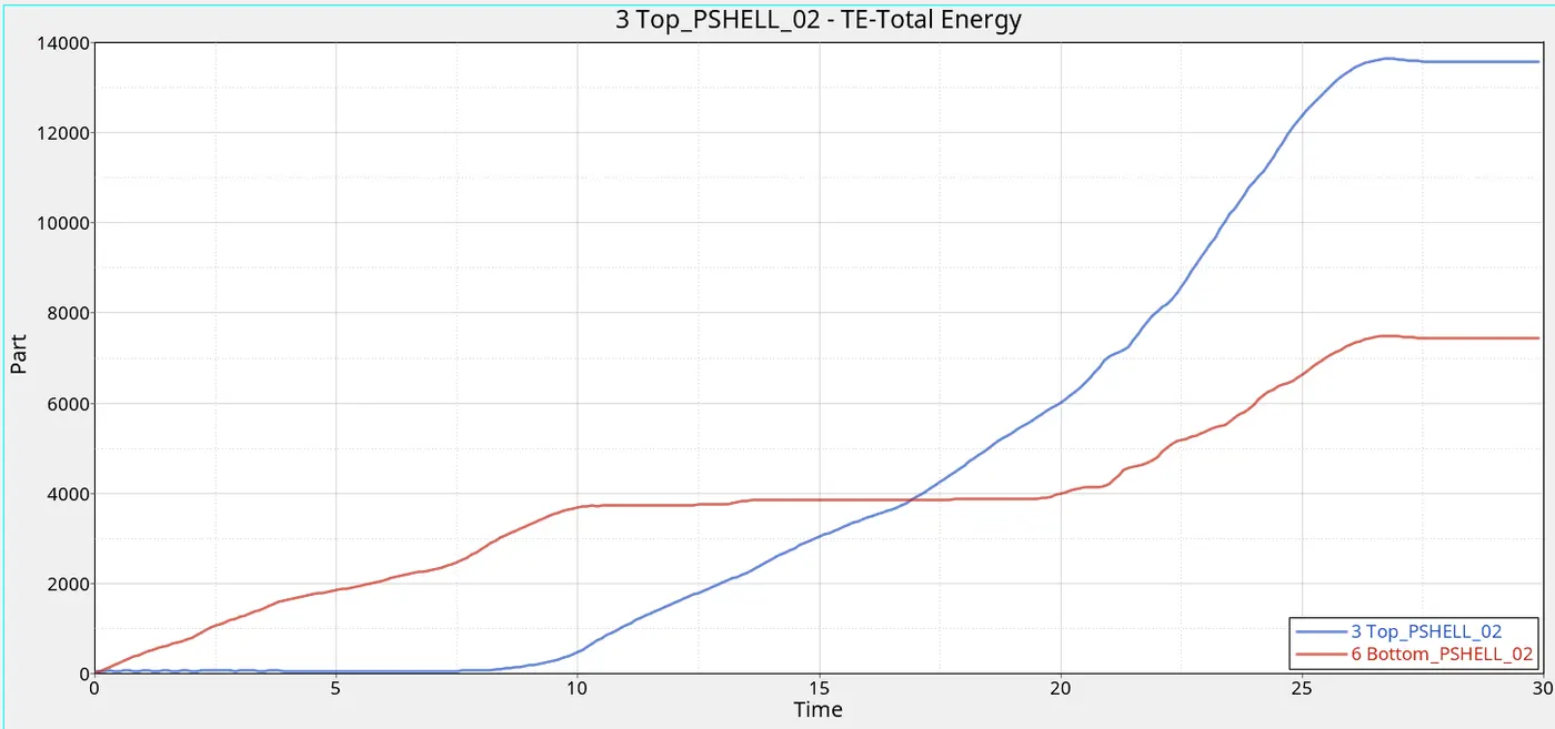
Plot 5,6: Time Vs Total Energies (Case 1)
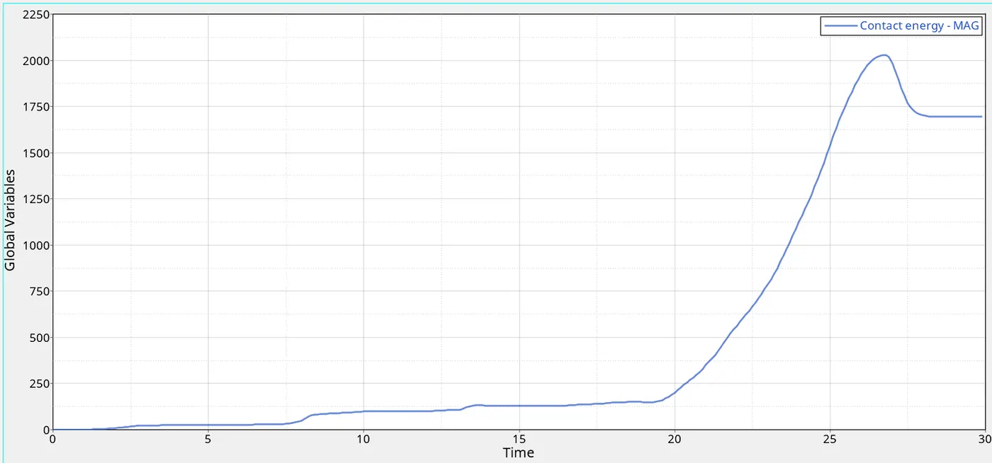
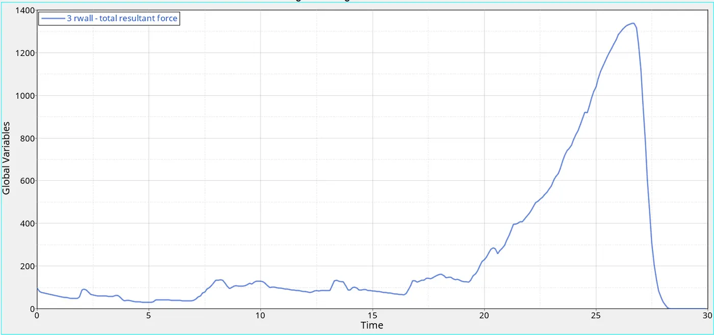
Plot 7: Time Vs Contact Energy (Case 1) Plot 8: Time Vs Total Resultant Forces (Case 1)
Case 2: Change the Inacti=6 and run.
Step 1: Setup Case Definitions
Import 'CrushTube_NoChanges_Case1_0000.rad' In case two, the simulation is done by changing the value of Inacti=6. For that, we have to go to the solver browser.
- Solver Browser >> INTER >> Type 7 >> Self Contact >> Inacti=6.
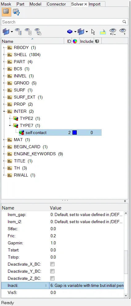
Fig 11: Changing Inacti=6
Step 2: Simulate the Model and Analysis of the Results
- Analysis >> Radioss >> Browse Input File Location >> Option = -nt 4 (No. Of Threads) >> Radioss
After that, run the simulation and save the file named 'Crush_tube_Inacti6_Case2_0000.rad'. Following previous methods, analyse the output file, and animations using Hyper View.
- Energy Error = -3.8%
- Mass Error = 0.0%
The errors are within the acceptable range. So we can continue with the model. Using the hyper view, we can make the contours with Von Mises Stress.
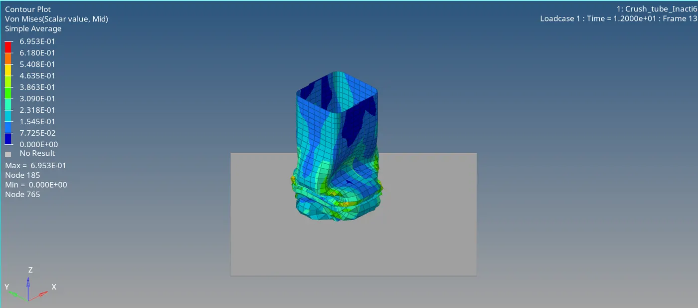
Fig 12: Contours- Von Mises Stress (Case 2)
Step 3: Plotting Necessary Graphs Using Hyper Graph 2D
The plots are drawn using the hypergraph 2D, by opening the Time History File of the model.
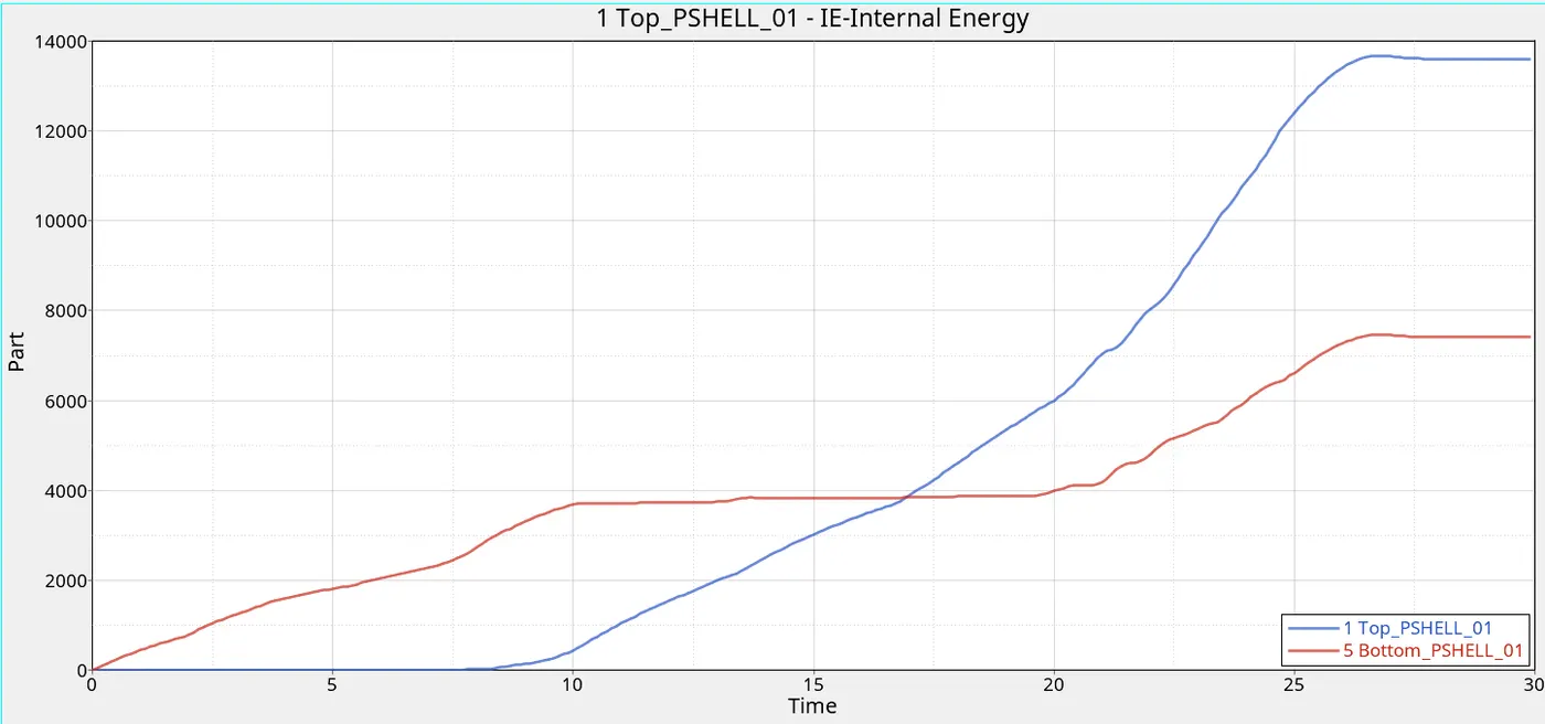
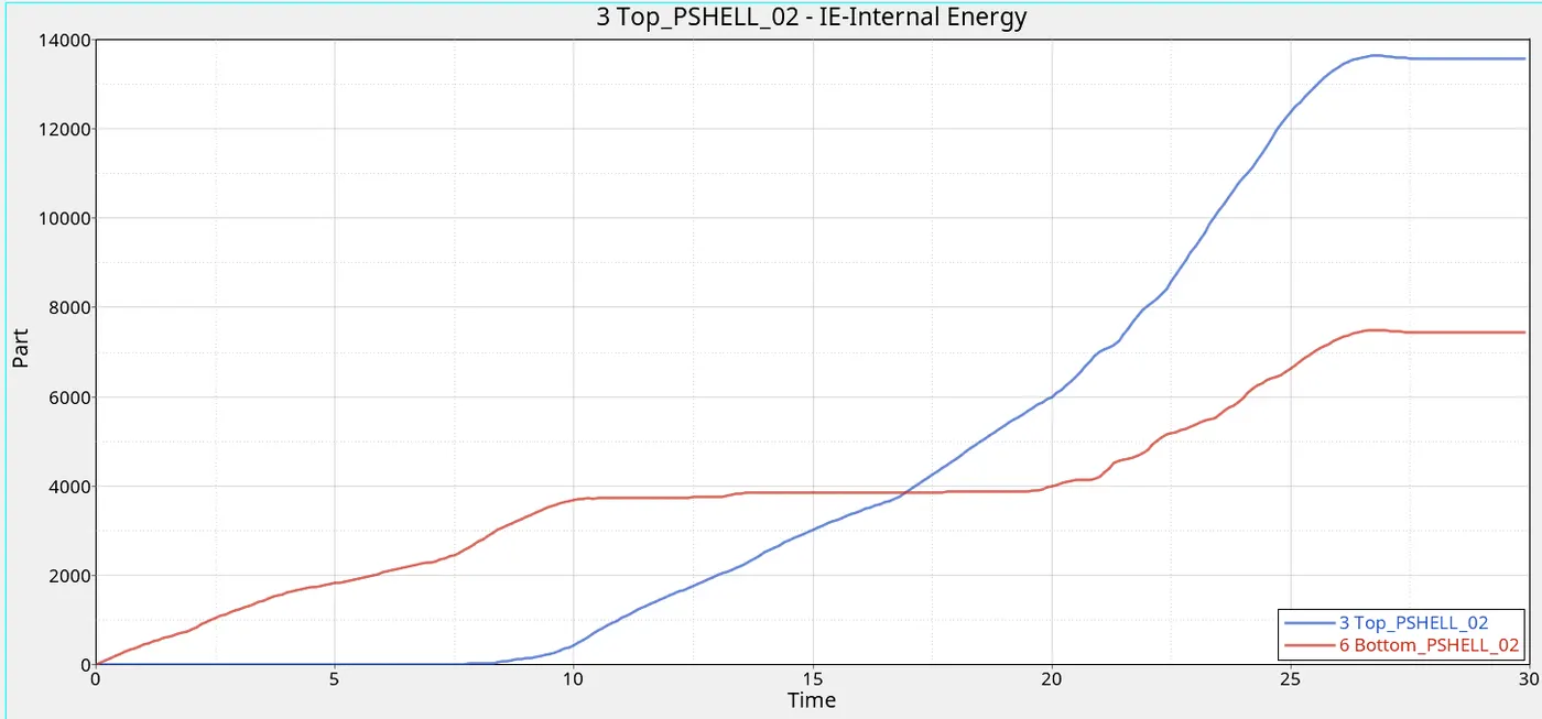
Plot 9,10: Time Vs Internal Energies (Case 2)
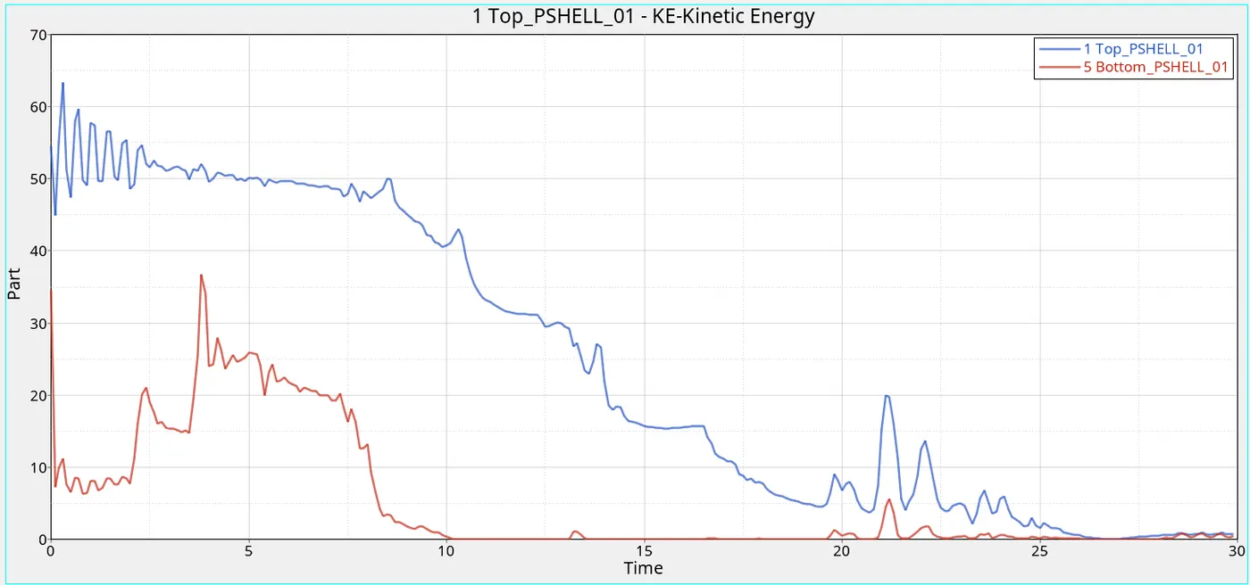
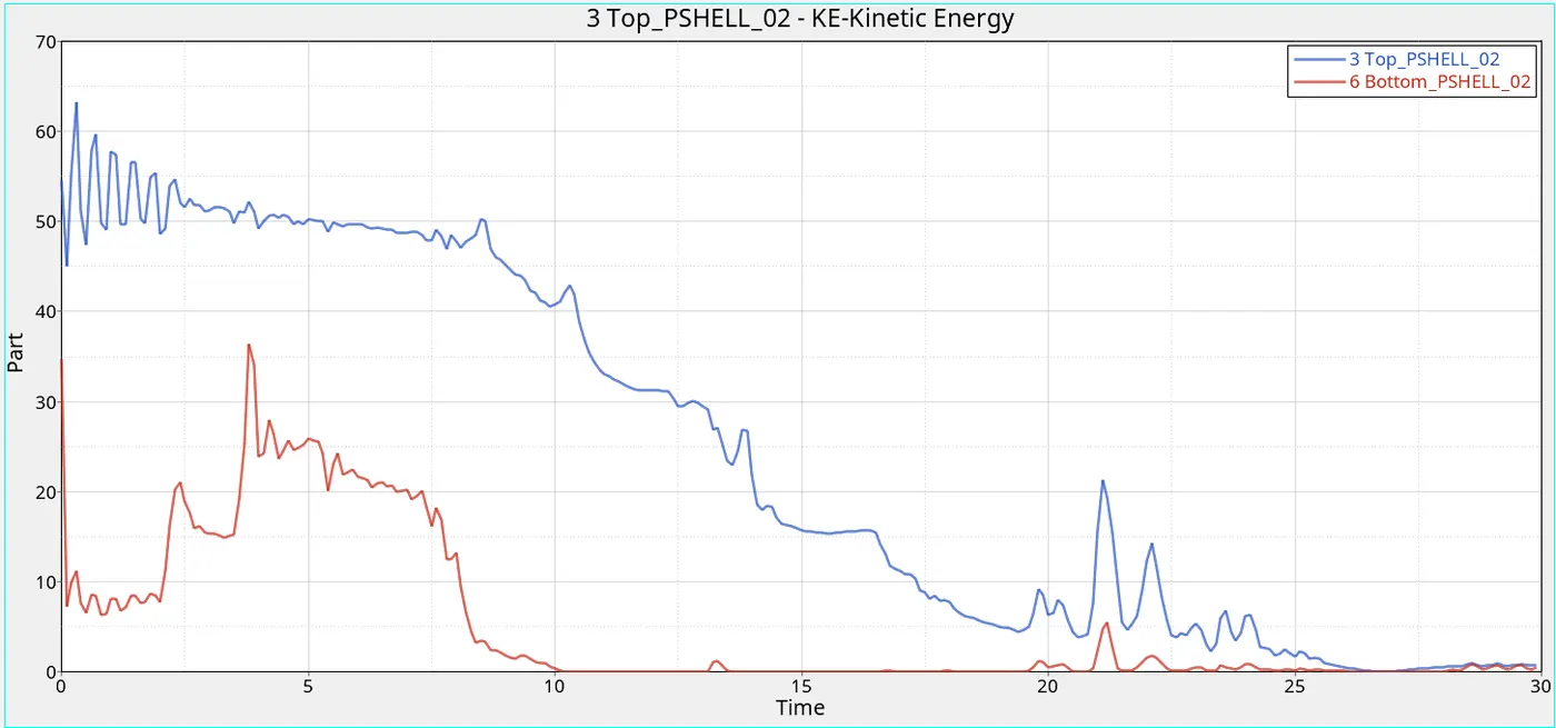
Plot 11,12: Time Vs Kinetic Energies (Case 2)
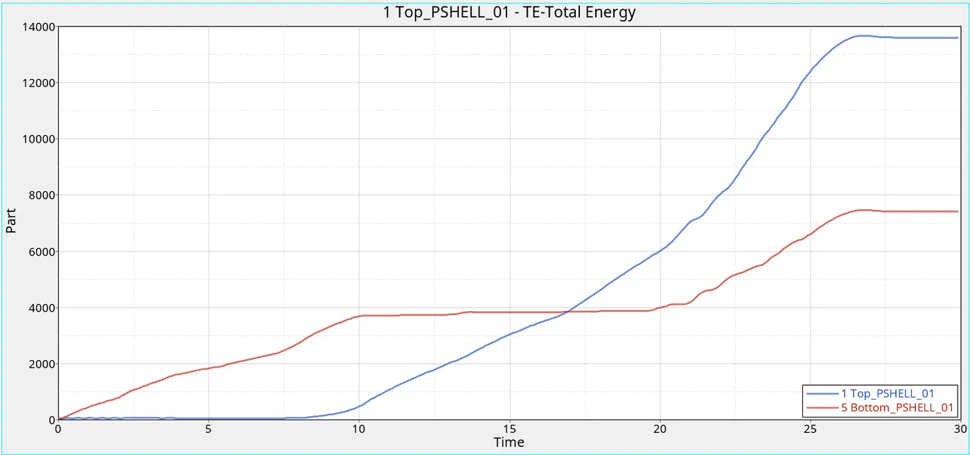
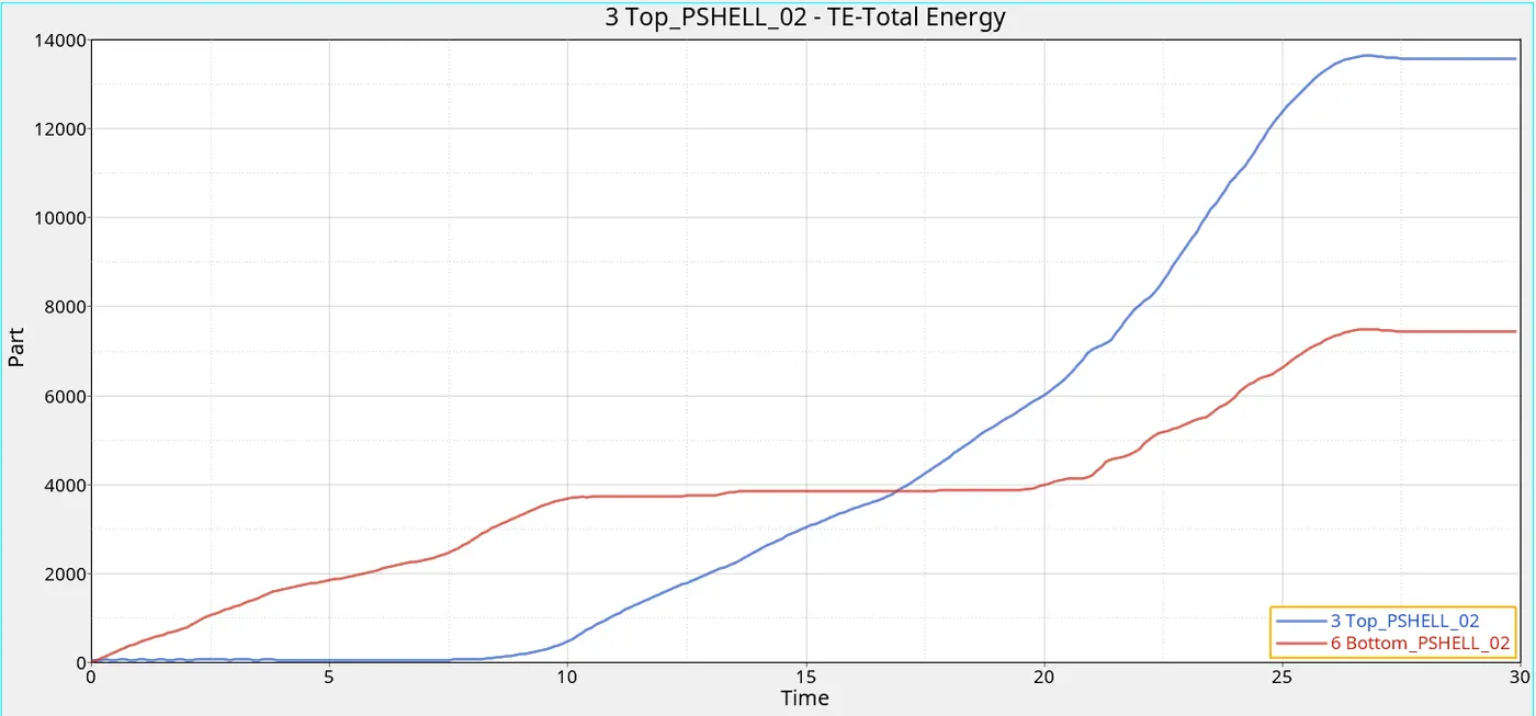
Plot 13,14: Time Vs Total Energies (Case 2)
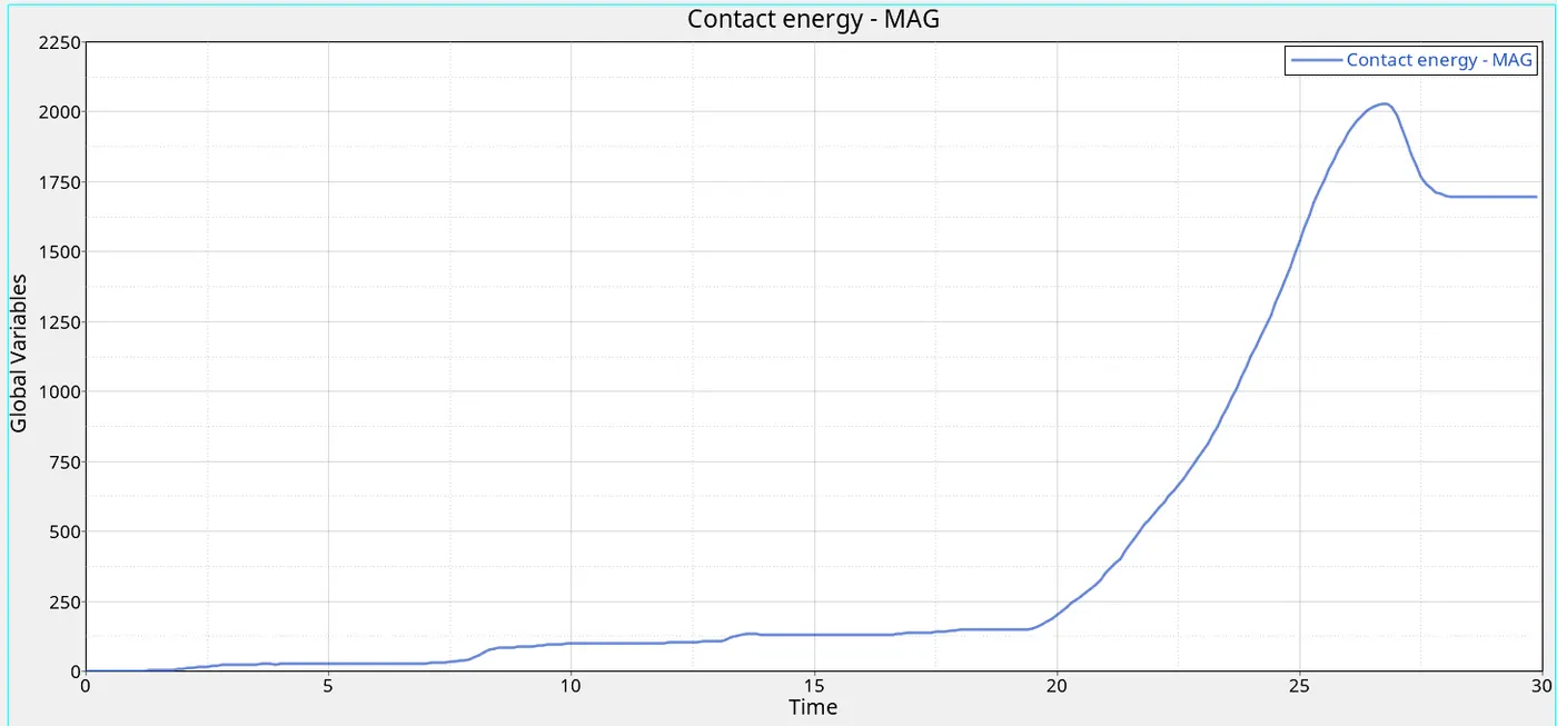
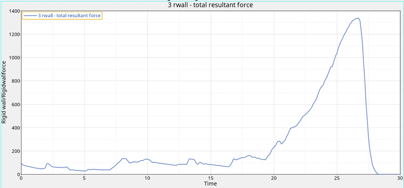
Plot 15: Time Vs Contact Energy (Case 2) Plot 16: Time Vs Total Resultant Forces (Case 2)
Case 3: Create the Type 11 contact and run.
Step 1: Setup Case Definitions
Import Crush_tube_Inacti6_Case2_0000.rad For this case, we have to define a Type 11 contact and assign all the recommended values. Type 11 can be created using the solver browser (INTER).
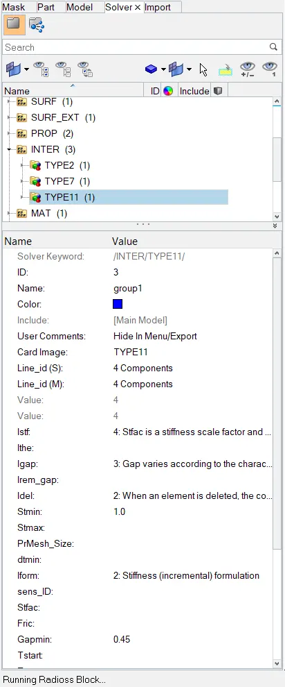
Fig13: Creating Type 11 Interface and Assigning Values.
Step 2: Simulate the Model and Analysis of the Results
- Analysis >> Radioss >> Browse Input File Location >> Option = -nt 4 (No. Of Threads) >> Radioss
After that, run the simulation and save the file named 'Crush_tube_Inacti6_Type11_Case3_0000.rad'. Following previous methods, analyse the output file, and animations using Hyper View.
-
- Energy Error = -1.7%
- Mass Error = 0.0%
The errors are within the acceptable range. So we can continue with the model. Using the hyper view, we can make the contours with Von Mises Stress.
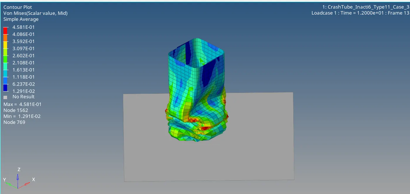
Fig 12: Contours- Von Mises Stress (Case 3)
Step 3: Plotting Necessary Graphs Using Hyper Graph 2D
The plots are drawn using the hypergraph 2D, by opening the Time History File of the model.
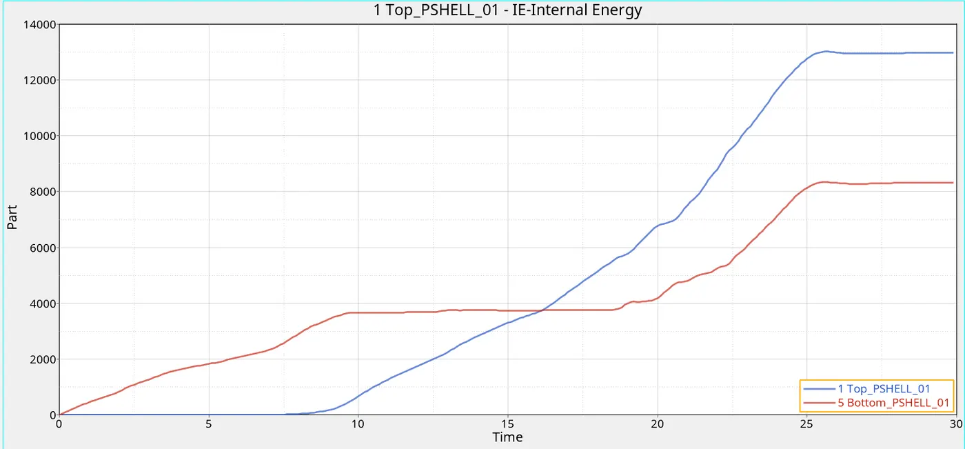
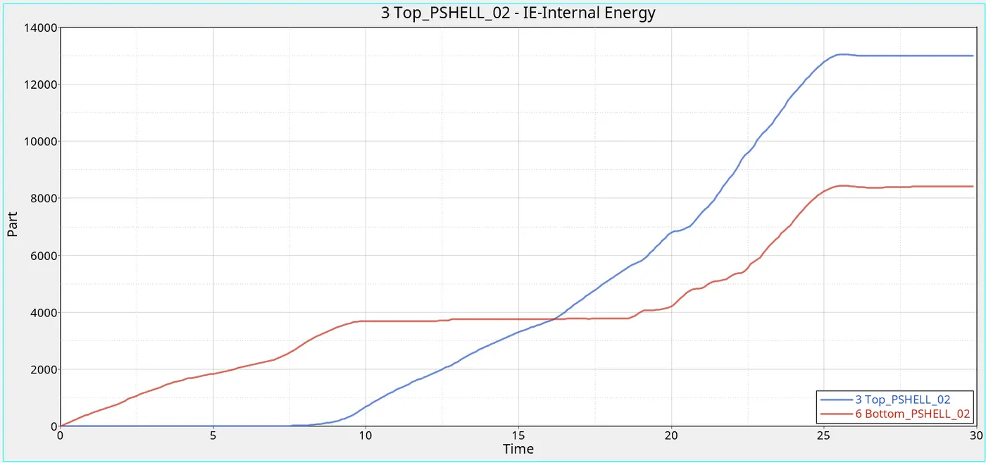
Plot 17,18: Time Vs Internal Energies (Case 3)
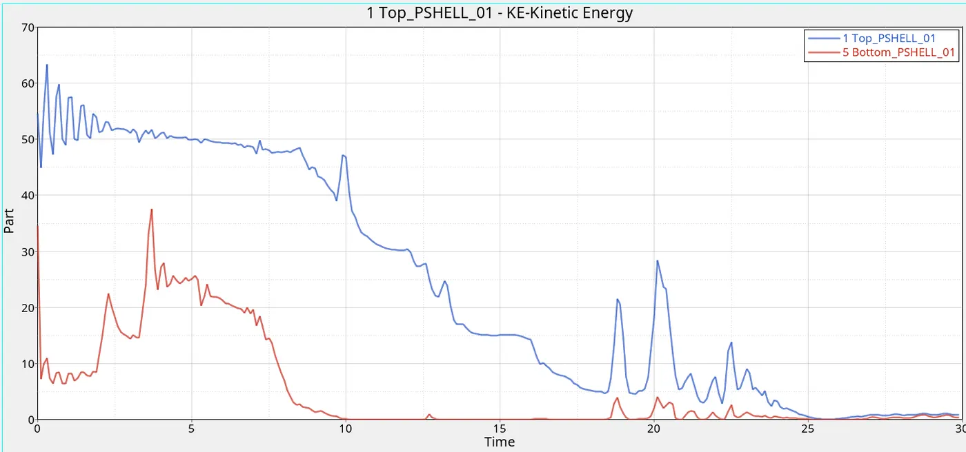
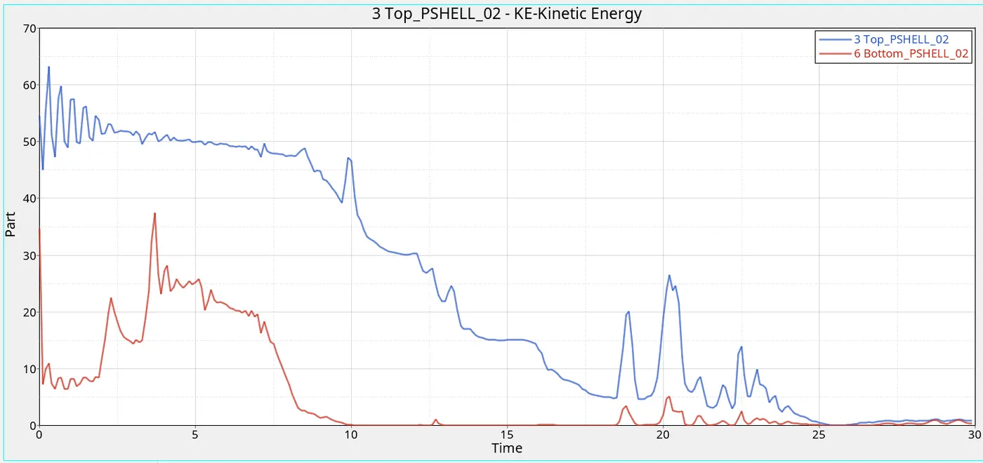
Plot 19,20: Time Vs Kinetic Energies (Case 3)
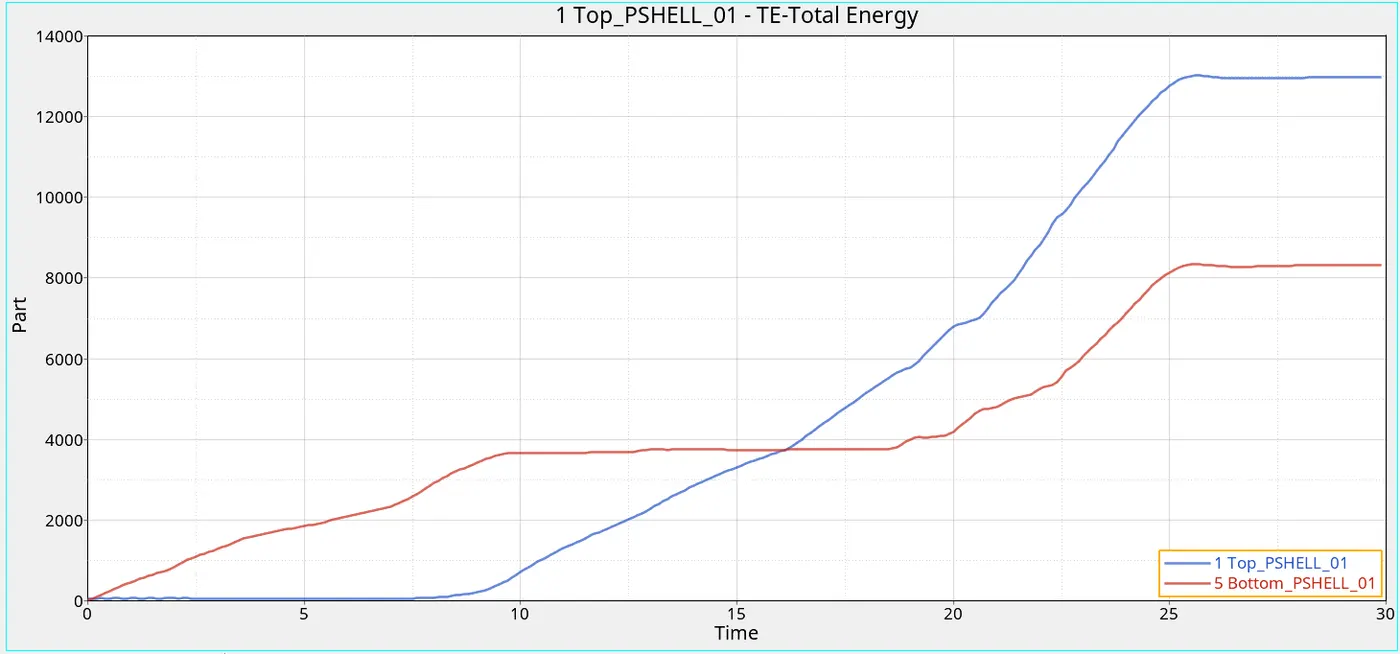
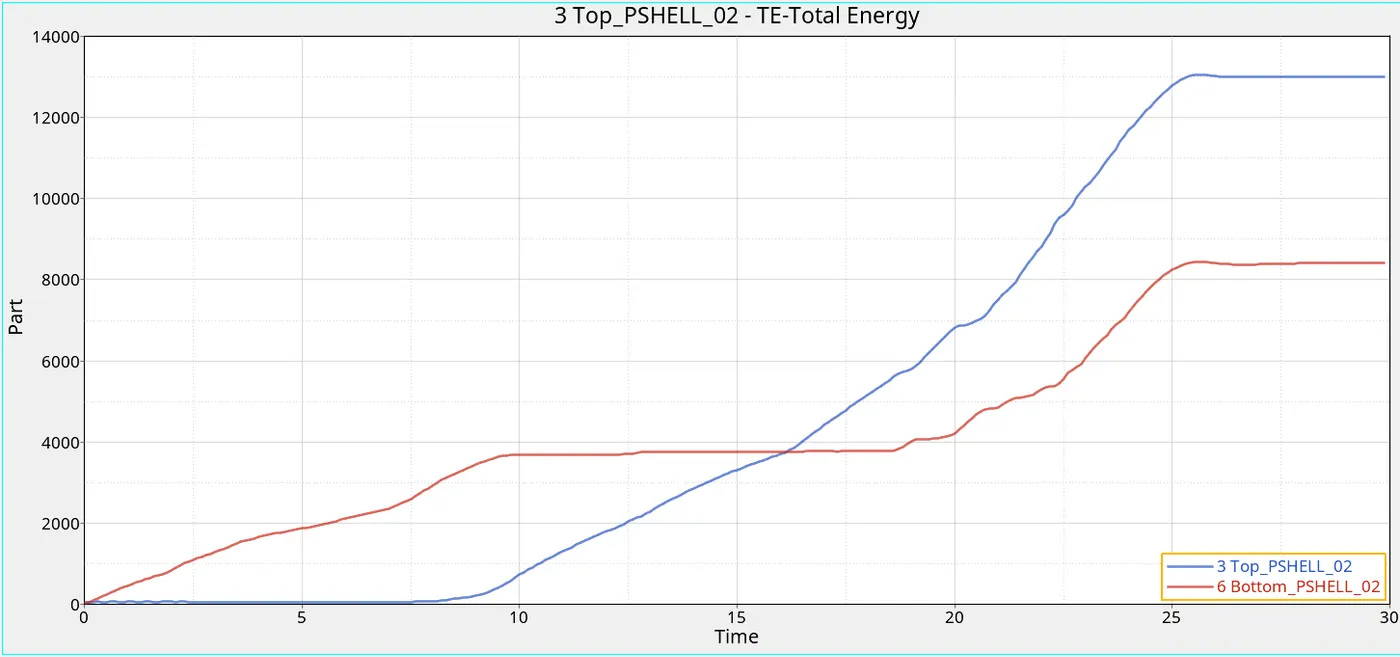
Plot 21,22: Time Vs Total Energies (Case 3)
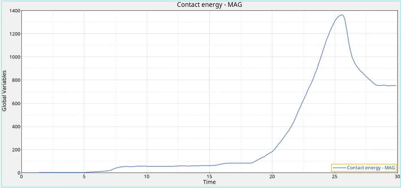
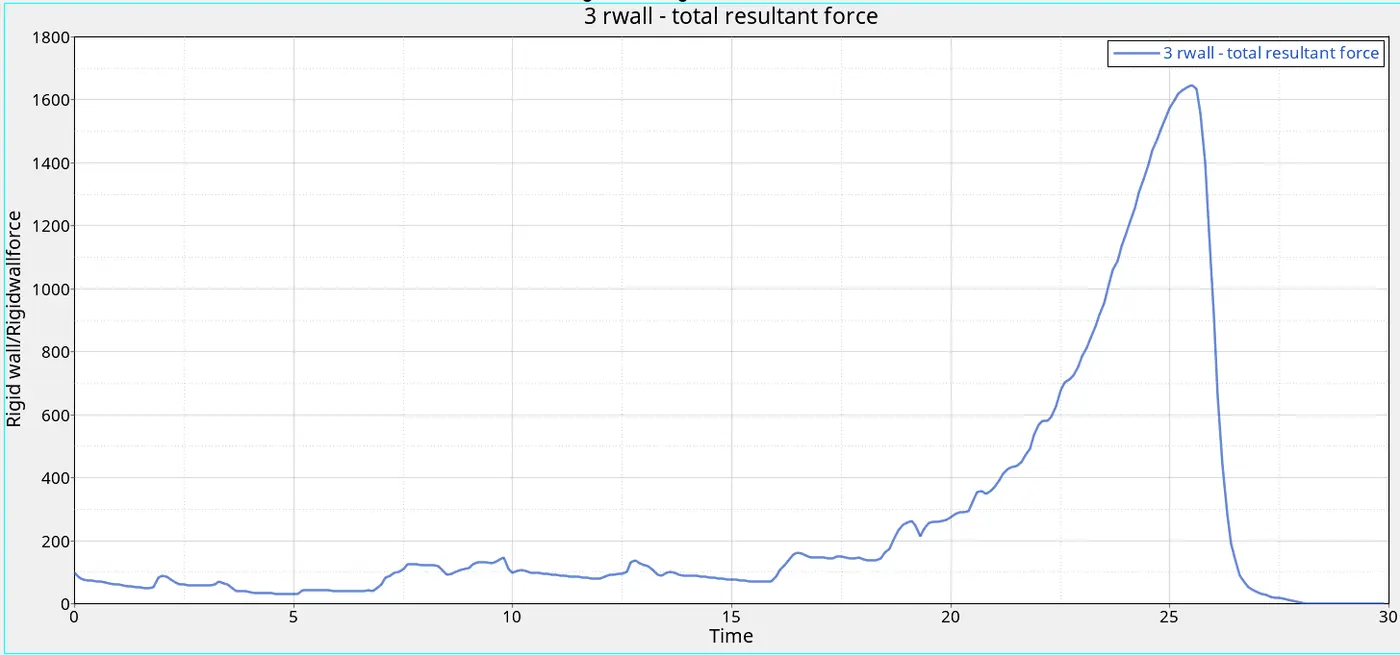
Plot 23: Time Vs Contact Energy (Case 3) Plot 24: Time Vs Total Resultant Forces (Case 3)
Case 4:- Remove both notches and remove boundary condition on rigid body node then run.
Step 1: Setup Case Definitions
Import Crush_tube_Inacti6_Case2_0000.rad. The notches can be removed by using various methods. Here we use the align command to allign the nodes and remove the notches from geometry.
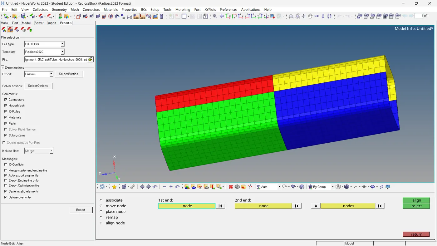
Fig 13: Removing Of Notches.
Then remove the boundary conditions by using the solver deck. Delete the BCS from the solver browser. Also, we can unselect the DOF constraints from the BCS.
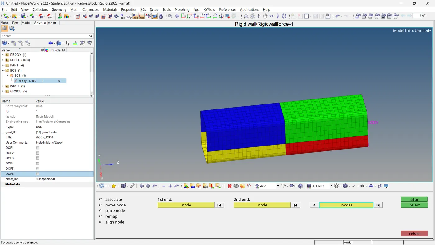
Fig 14: Removing Of Boundary Conditions.
Step 2: Simulate the Model and Analysis of the Results
- Analysis >> Radioss >> Browse Input File Location >> Option = -nt 4 (No. Of Threads) >> Radioss
After that, run the simulation and save the file named 'CrashTube_Inacti6_NoNotch_NoBCS_Case_4_0000.rad'.' analyse the output file, and animations using Hyper View.
- Energy Error = -3.1%
- Mass Error = 0.0%
The errors are within the acceptable range. So we can continue with the model. Using the hyper view, we can make the contours with Von Mises Stress.
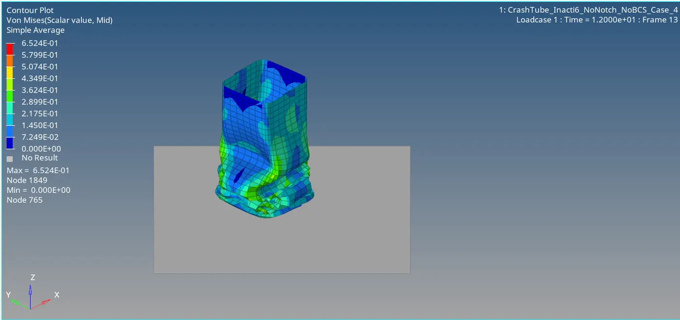
Fig 15: Contours- Von Mises Stress (Case 4)
Step 3: Plotting Necessary Graphs Using Hyper Graph 2D
The plots are drawn using the hypergraph 2D, by opening the Time History File of the model.
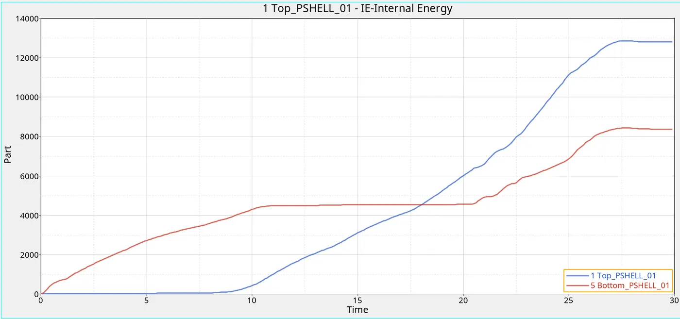
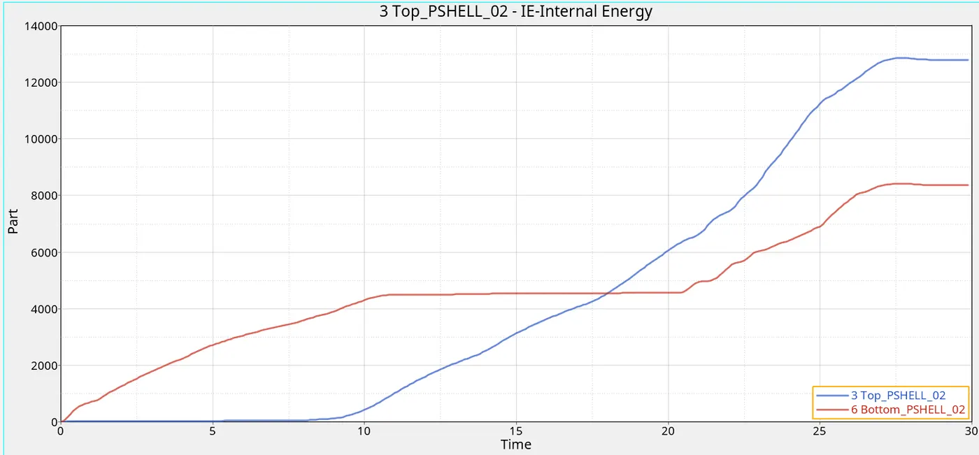
Plot 25,26: Time Vs Internal Energies (Case 4)
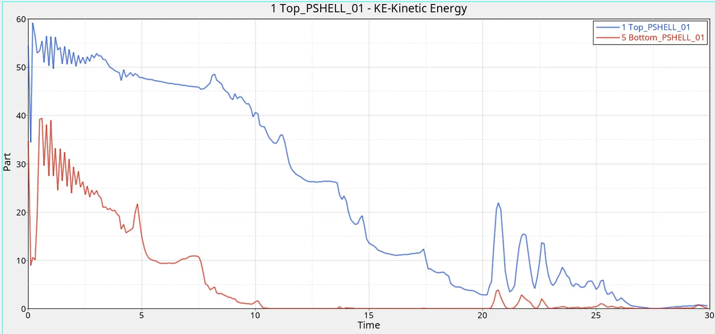
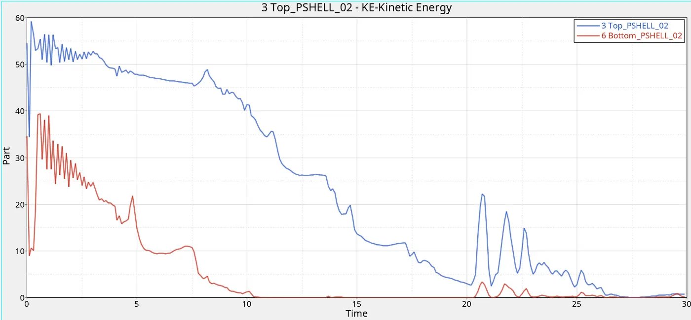
Plot 27,28: Time Vs Kinetic Energies (Case 4)
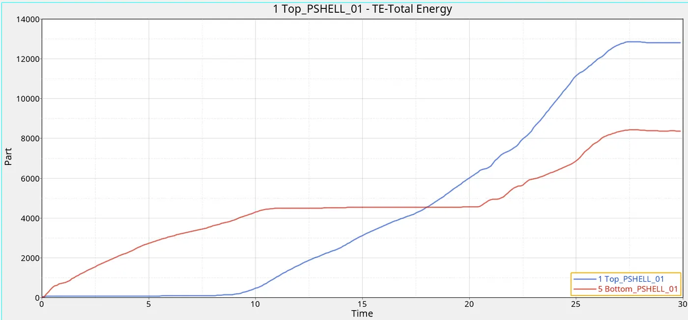
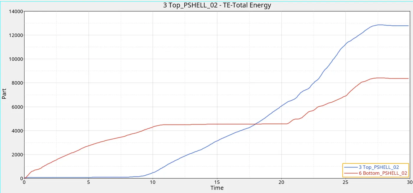
Plot 29,30: Time Vs Total Energies (Case 4)
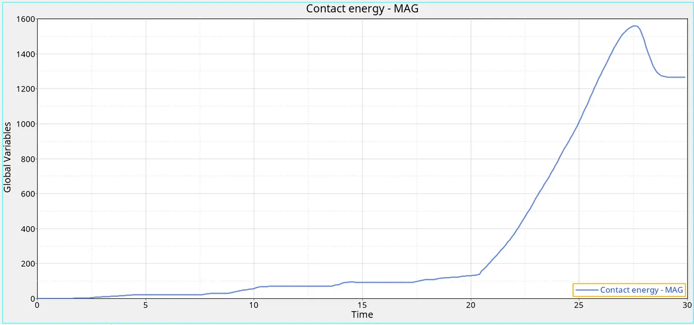
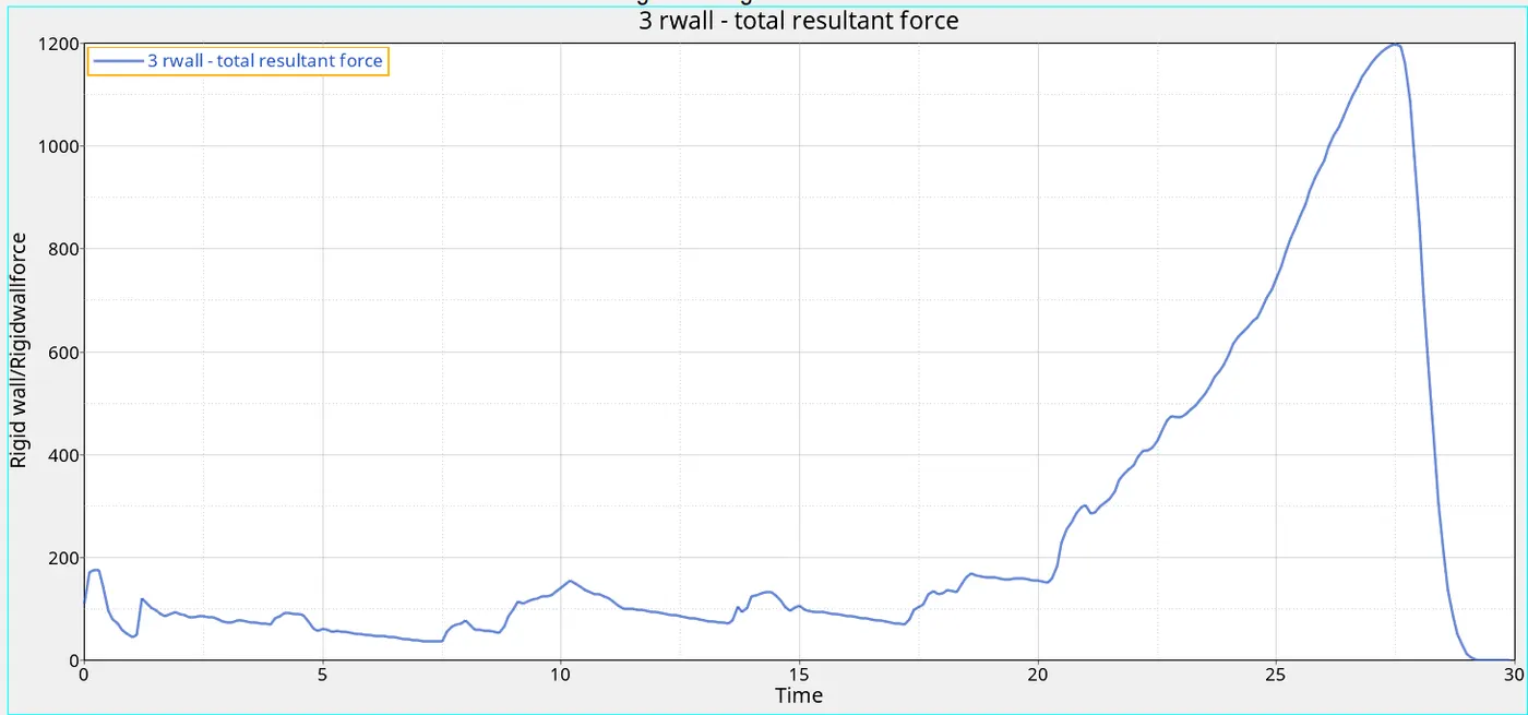
Plot 31: Time Vs Contact Energy (Case 4) Plot 32: Time Vs Total Resultant Forces (Case 4)
Case 5: Create a new notch in the middle, select the whole section and run.
Step 1: Setup Case Definitions
Here we have to create a notch with a depth of 3mm in the middle of the crash tube. we can use the translate option to make notches. Remove the DOF constraints from the boundary conditions. The interface Type is Type 7. Import 'CrashTube_Inacti6_NoNotch_NoBCS_Case_4_0000.rad'
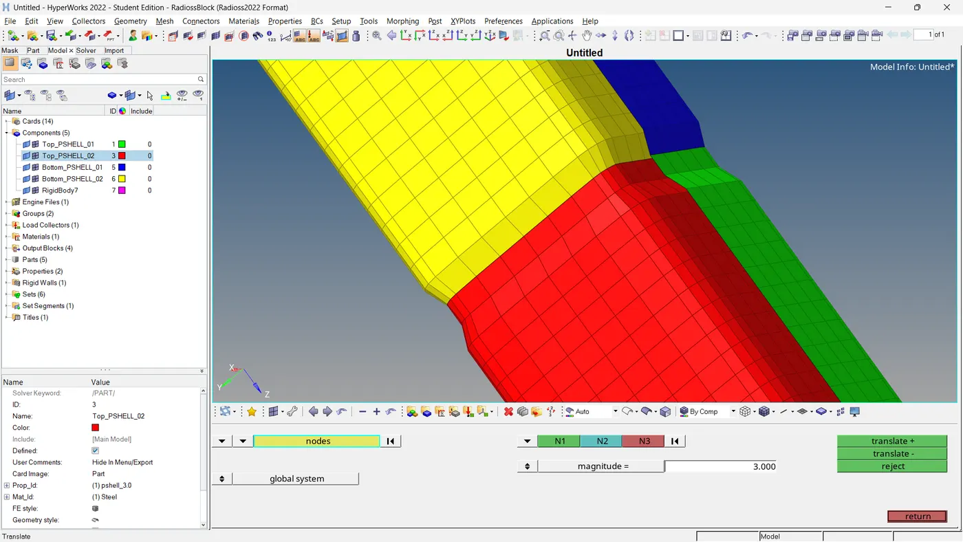
Fig 16: Creating Notches Using Translate Option
Step 2: Simulate the Model and Analysis of the Results
- Analysis >> Radioss >> Browse Input File Location >> Option = -nt 4 (No. Of Threads) >> Radioss
After that, run the simulation and save the file named 'CrashTube_Inacti6_MidNotch_NoBCS_Case_5_0000.rad'.' analyse the output file, and animations using Hyper View.
- Energy Error = -3.7%
- Mass Error = 0.0%
The errors are within the acceptable range. So we can continue with the model. Using the hyper view, we can make the contours with Von Mises Stress.
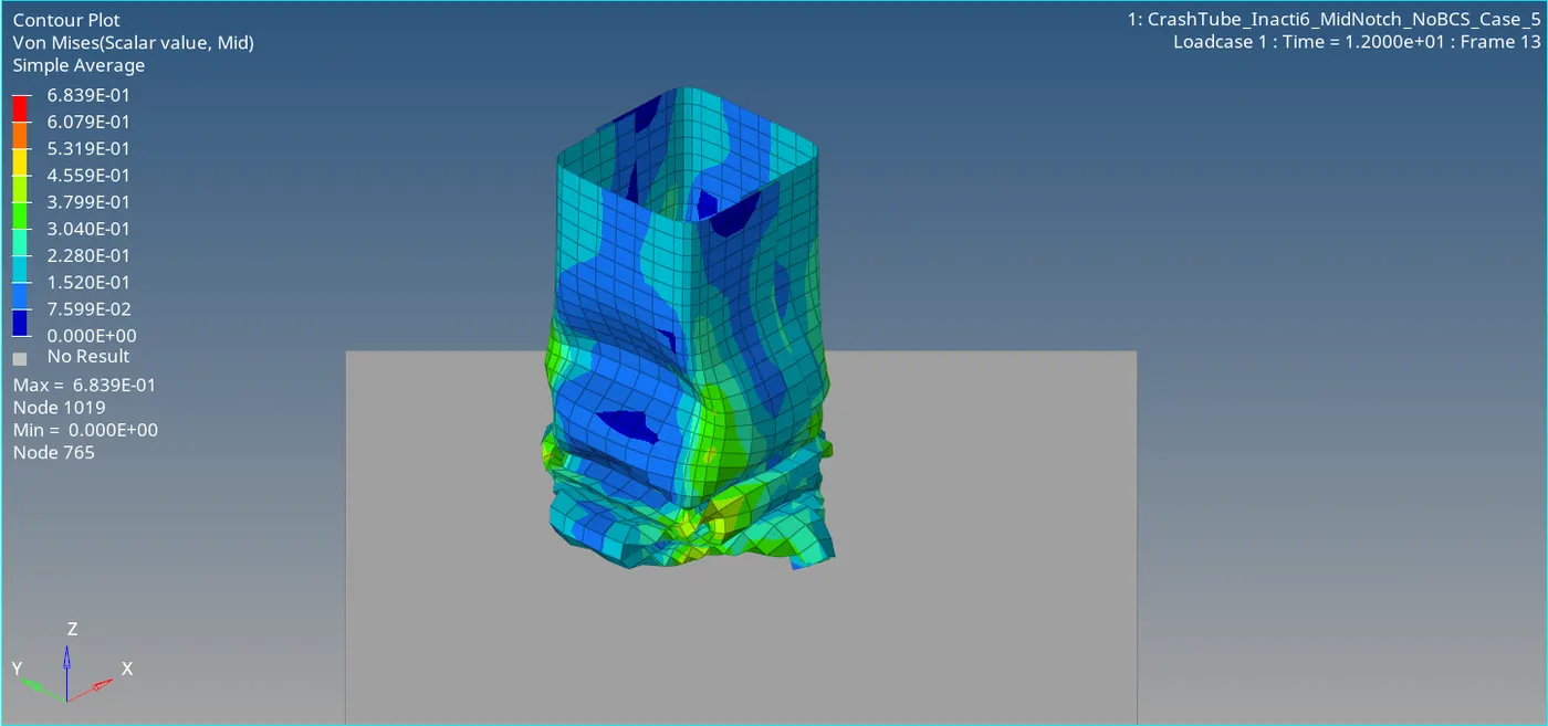
Fig 17: Contours- Von Mises Stress (Case 5)
Step 3: Plotting Necessary Graphs Using Hyper Graph 2D
The plots are drawn using the hypergraph 2D, by opening the Time History File of the model.
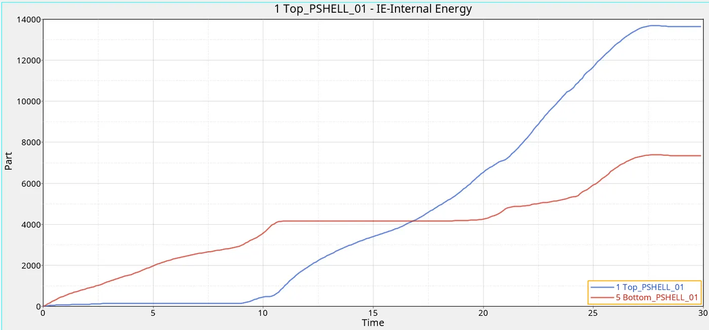
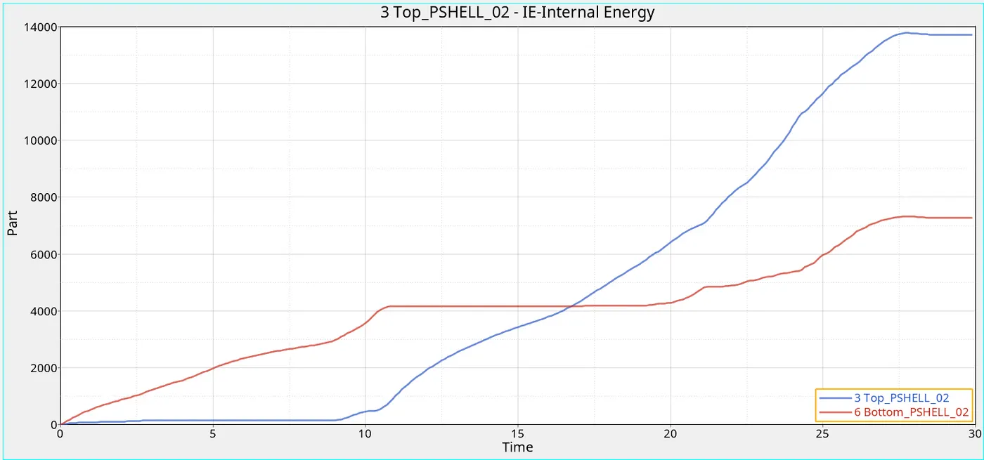
Plot 33,34: Time Vs Internal Energies (Case 5)
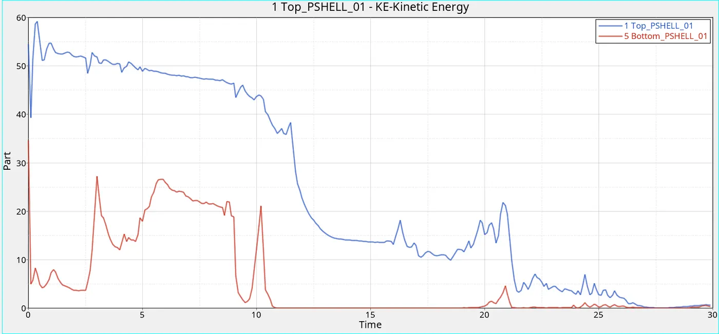
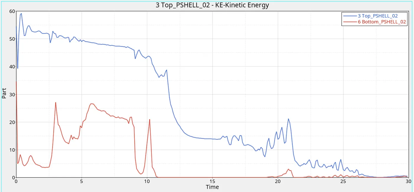
Plot 35,36: Time Vs Kinetic Energies (Case 5)
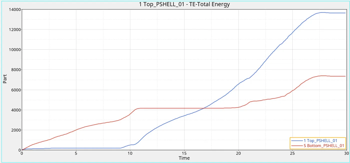
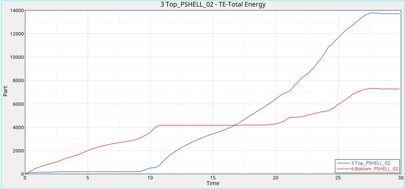
Plot 37,38: Time Vs Total Energies (Case 5)
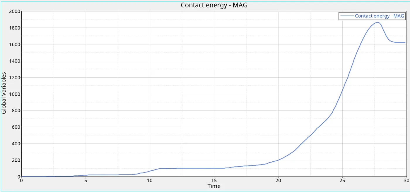
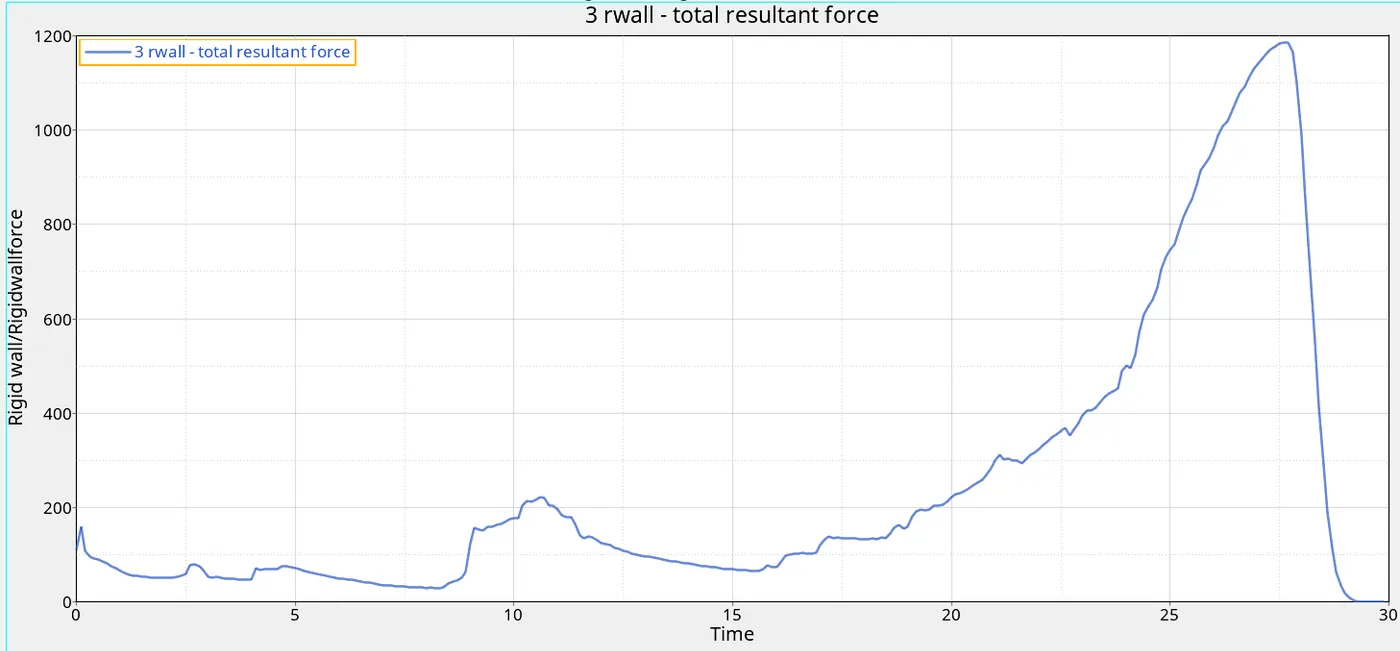
Plot 39: Time Vs Contact Energy (Case 5) Plot 40: Time Vs Total Resultant Forces (Case 5)
Case 6: Create a new notch with nodes only from opposing 2 faces and run.
In this case, we have to create a new notch (in the middle of the crash tube) with nodes only from opposing two faces. Import CrashTube_Inacti6_NoNotch_NoBCS_Case_4_0000.rad. Then create a new notch having a depth of 3mm. It is done by using the translate option.
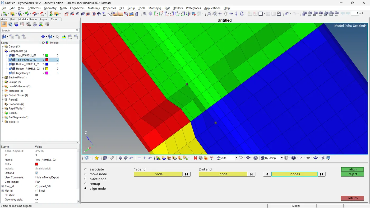
Fig 18: Creating New Notches Using Translate Option
Step 2: Simulate the Model and Analysis of the Results
- Analysis >> Radioss >> Browse Input File Location >> Option = -nt 4 (No. Of Threads) >> Radioss
After that, run the simulation and save the file named 'CrashTube_Inacti6_MidNotchHalf_NoBCS_Case_6_0000.rad'.' analyse the output file, and animations using Hyper View.
- Energy Error = -2.8%
- Mass Error = 0.0%
The errors are within the acceptable range. So we can continue with the model. Using the hyper view, we can make the contours with Von Mises Stress.
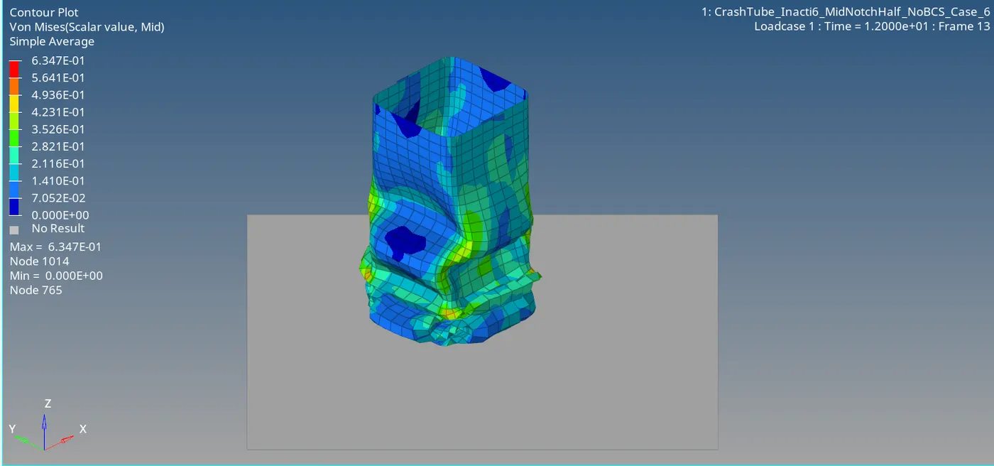
Fig 19: Contours- Von Mises Stress (Case 6)
Step 3: Plotting Necessary Graphs Using Hyper Graph 2D
The plots are drawn using the hypergraph 2D, by opening the Time History File of the model.
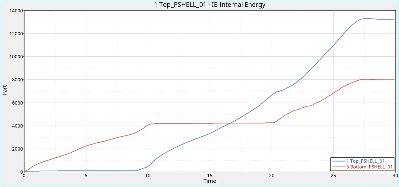
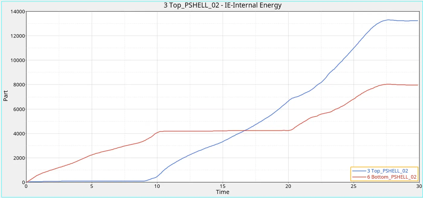
Plot 41,42: Time Vs Internal Energies (Case 6)
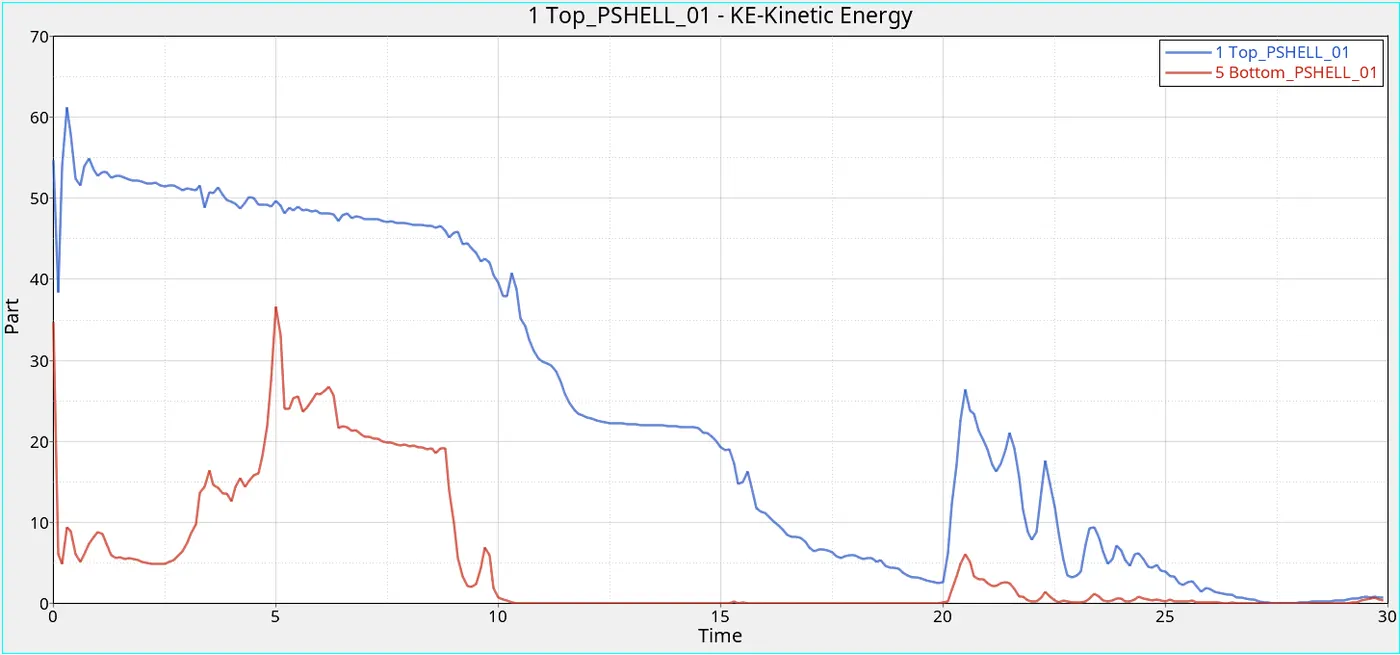
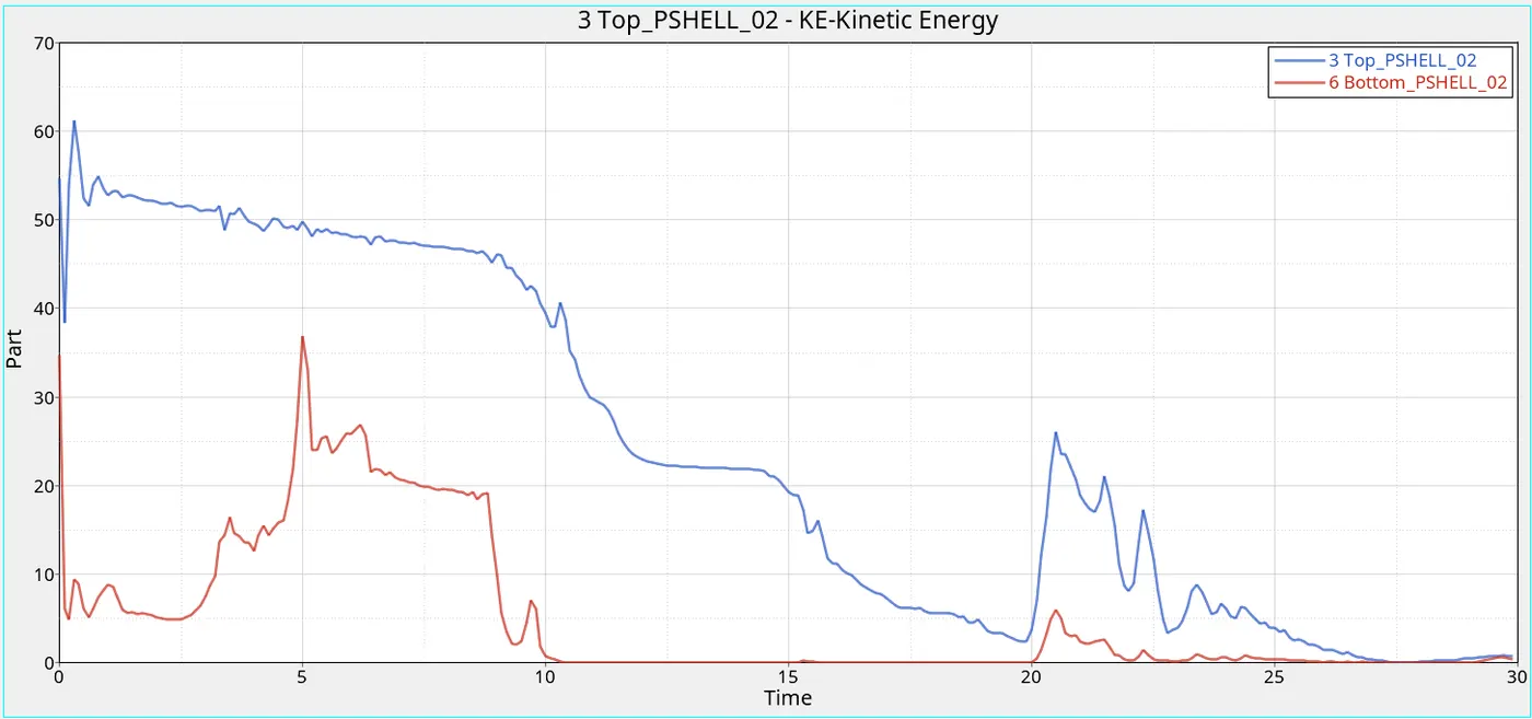
Plot 43,44: Time Vs Kinetic Energies (Case 6)
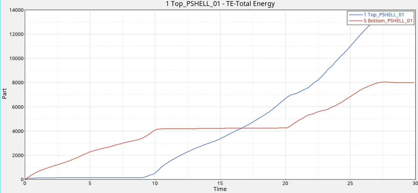
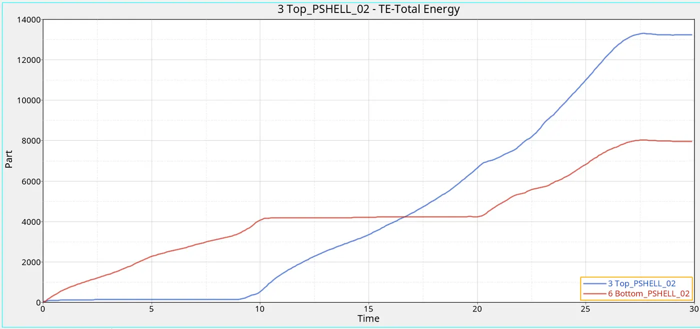
Plot 45,46: Time Vs Total Energies (Case 6)
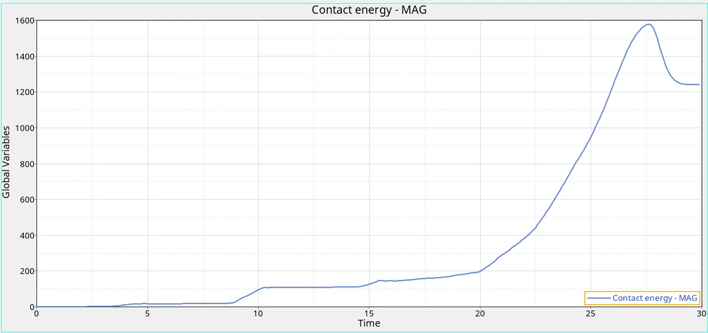
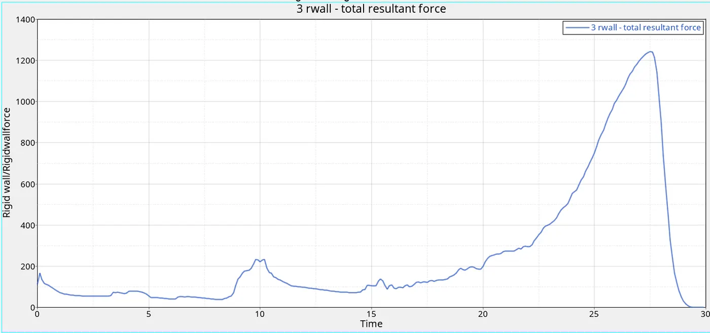
Plot 47: Time Vs Contact Energy (Case 6) Plot 48: Time Vs Total Resultant Forces (Case 6)
4. Observation
For an easy comparison, the results of each simulation are tabulated below.
| No. | Simulation Name/File Name | Case Description | Interface Types | Boundary Condition | Simulation Time (Sec) | Total No. of Cycles | Energy Error | Mass Error | Maximum Stress (Acting Node No) |
| 1 |
CrushTube_NoChanges_Case1_0000.rad |
Run the crash tube model as it is. | Type 2 / Type 7 | Y | 70.30 | 83469 | -3.8% | 0.0 | 6.953E-01 (185) |
| 2 |
CrushTube_Inacti6_Case2_0000.rad |
Change the Inacti=6 and run. | Type 2 / Type 7 | Y | 71.40 | 83469 | -3.8% | 0.0 | 6.953E-01 (185) |
| 3 | CrushTube_Inacti6_Type11_Case3_0000.rad |
Create the Type 11 contact and run. |
Type 2 / Type 7 / Type 11 | Y | 212.94 | 105615 | -1.7% | 0.0 | 4.581E-01 (1562) |
| 4 | CrashTube_Inacti6_NoNotch_NoBCS_Case_4_0000.rad | Remove both notches and remove boundary condition on rigid body node then run. |
Type 2 / Type 7 |
N | 68.73 | 78435 | -3.0% | 0.0 | 6.524E-01 (1849) |
| 5 | CrashTube_Inacti6_MidNotch_NoBCS_Case_5_0000.rad | Create a new notch in the middle, select the whole section and run. |
Type 2 / Type 7 |
N | 74.34 | 86332 | -3.7% | 0.0 | 6.839E-01 (1019) |
| 6 | CrashTube_Inacti6_MidNotchHalf_NoBCS_Case_6_0000.rad | Create a new notch with nodes only from opposing 2 faces and run. |
Type 2 / Type 7 |
N | 61.46 | 70134 | -2.8% | 0.0 | 6.347E-01 (1014) |
Table 2: Comparison Between Each Case
Case 1
- For internal energy, for the top shell (3mm), the IE increases at around 09ms whereas for the bottom shell (2mm) it starts to rise at the beginning 0ms. It is because in the simulation, the bottom part comes into contact initially and the effects of the collision lead to an increase in IE. From 10ms to 20ms the graph keeps a steady rate then it increases to its peak value till the end of the simulation. whereas the top part only compresses after 11ms, so the increase in IE rises after that time. The value of internal energy is higher for top components than for bottom components.
- For kinetic energy, for the bottom shell (2mm) the deformation occurs for the first 10ms, and we can see that the graph is maintained as constant because all deformations are done in the first 10ms. But if we consider the top shell (3mm), it has changed in KE up to 25ms. The deformations came into contact after the first 25ms then it went to around a constant ~0 value. The presence of notches also helps the bottom part to deform rapidly. The rate of kinetic energy is higher in the top components. However rapid deformations take place in bottom components. The presence of notches also leads to a rapid drop of kinetic energy in the bottom part. There is no effect of notches presence in the top part.
- The contact energy is increased with a small limit up to the start of deformation, and then a sudden peak of energy is created at the end of the deformation.
- For the rigid wall, the graphs went to small up and downs up to 17ms and gradually increased the maximum limit of contact energy (Time~26ms) then rapidly fell to zero as the deformation ended.
Case 2
- The characteristics of each graph are same as the case 1. Here we changed the value of Inacti=6, where it describes the gap is reduced and scaled to avoid the initial penetrations. It provides good accuracy for the results.
- The total number of cycles, mass error, energy error, and maximum stress is the same as in the previous case.
Case 3
- Here we provide a new interface, that is Type 11- Edge to Edge contact. It can tolerate the intersection between master segments and slave nodes. It is defined by the master and slave lines. For internal energy, the bottom shell (2mm) starts to deform at the beginning of simulation causing the rise in internal energy from 0ms itself. From 10ms to 20ms the graph keeps a steady rate then it increases to its peak value till the end of the simulation. The top shell has a thickness of 3mm and for this component, the deformation starts at 9ms, so the rise in internal energy only begins from that point. The value of internal energy is higher for top components than for bottom components.
- Because the initial contact takes place in the bottom part, the kinetic energy comes to zero point in the first 10ms. The notches also help with this rapid deformation. For the top shell, it has changed in kinetic energy up to 25ms. The deformations came into contact after the first 25ms then it went to around a constant ~0 value. The rate of kinetic energy is higher in the top components. However rapid deformations take place in bottom components. The presence of notches also leads to a rapid drop of kinetic energy in the bottom part. There is no effect of notches presence in the top part.
- The contact energy is increased with a small limit up to the start of deformation, and then a sudden peak of energy is created at the end of the deformation.
- For the rigid wall, the graphs went to small up and downs up to 17ms and gradually increased the maximum limit of contact energy(Time~26ms) then rapidly fell to zero as the deformation ended.
Case 4
- Here the notches are removed. So there is no influence of notches in deformation.
- The internal energy of the bottom shell (2mm) starts to deform at the beginning of simulation causing the rise in internal energy from 0ms itself. From 10ms to 20ms the graph keeps a steady rate then it increases to its peak value till the end of the simulation. The top shell has a thickness of 3mm and for this component, the deformation starts at 9ms, so the rise in internal energy only begins from that point. The value of internal energy is higher for top components than for bottom components.
- For the bottom part, the kinetic energy comes to zero point in the first 10ms. For the top shell, it has changed in kinetic energy up to 25ms. The deformations came into contact after the first 25ms then it went to around a constant ~0 value. The rate of kinetic energy is higher in the top components. However rapid deformations take place in bottom components. In the case of bottom components, there are no rapid drops in the kinetic energies due to the notches.
- The contact energy is increased with a small limit up to the start of deformation, and then a sudden peak of energy is created at the end of the deformation.
- For the rigid wall, the graphs went to small up and downs up to 17ms and gradually increased the maximum limit of contact energy (Time~26ms) then rapidly fell to zero as the deformation ended.
Case 5
- Here the effects of a middle notch affect the deformation rate of both components.
- The internal energy of the bottom shell (2mm) starts to deform at the beginning of simulation causing the rise in internal energy from 0ms itself. From 10ms to 20ms the graph keeps a steady rate then it increases to its peak value till the end of the simulation. The top shell has a thickness of 3mm and for this component, the deformation starts at 9ms, so the rise in internal energy only begins from that point. The value of internal energy is higher for top components than for bottom components.
- Here because the notches lie at the junction of both components, the effects come into the picture in both cases. For the bottom part, the notches are present at the end, which means the end of deformation, and we can see that at the end of a rapid drop of kinetic energy because of this notch. But at the same time, there is a drop in the kinetic energy present in the top section. The majority portion of notches lies on the top part, the effects of notches are high in kinetic energy of the top section.
- The contact energy is increased with a small limit up to the start of deformation, and then a sudden peak of energy is created at the end of the deformation.
- For the rigid wall, the graphs went to small up and downs up to 17ms and gradually increased the maximum limit of contact energy (Time~26ms) then rapidly fell to zero as the deformation ended.
Case 6
- Here the notch is created with nodes only from opposing 2 faces. But it lies on both the top and bottom sections.
- For internal energy, for the top shell (3mm), the IE increases at around 09ms whereas for the bottom shell (2mm) it starts to rise at the beginning 0ms. It is because in the simulation, the bottom part comes into contact initially and the effects of the collision lead to an increase in IE. From 10ms to 20ms the graph keeps a steady rate then it increases to its peak value till the end of the simulation. whereas the top part only compresses after 11ms, so the increase in IE rises after that time. The value of internal energy is higher for top components than for bottom components.
- Here the size and effects of notches are less and it leads to changes in both top and bottom parts. The effects are present in both cases, but not as much as in the previous case. Here also the majority portion of notches lies on the top part, the effects of notches are high in kinetic energy of the top section.
- The contact energy is increased with a small limit up to the start of deformation, and then a sudden peak of energy is created at the end of the deformation.
- For the rigid wall, the graphs went to small up and downs up to 17ms and gradually increased the maximum limit of contact energy (Time~26ms) then rapidly fell to zero as the deformation ended.
5. Results
- For the bumper model, meshing is done using the specified target element length and proper connections are made using suitable connectors.
- For the crush tube file, simulate each case and point out the effects of notches, interfaces, and interface parameters using necessary plots.