Challenge

Assignment 5-RADIOSS Interfaces & Study of Effect of Notches Challenge

RRavi Prasad20 Mar 2023

HTML RADIOSS

Assignment 5-RADIOSS Interfaces & Study of Effect of Notches Challenge

Aim -

To run the crash tube model by using different types of contact interfaces.
Mesh the given crash tube model with a 6mm size.

Objective -

Run the crash tube model with and without changing the parameters.
Remove the notches from the crash tube model, Remove the boundary conditions from rigid body node, and then run the simulation.
Create notches in the middle and in the opposing faces of the crash tube model and then run the simulation.
Perform geometry cleanup on the bumper assembly and mesh the bumper assembly with a 6mm size.

Theoretical Framework -

What is Hypermesh and Hypercrash ?

Hypermesh :

Hypermesh is a generalized preprocessor for many solvers like Abaqus,LS DYNA etc.,
In hypermesh,we can setup loadcases for Optistruct,Abaqus,ANSYS including Radioss and LS DYNA.

Hypercrash :

Hypercrash is a specialized preprocessor for radioss.It always exsist as a part of Hyperworks.Hypercrash is mainly used for crash applications.
Hypercrash supports solvers like Radioss and LS DYNA.The units used in industries are kn,mm,ms,kg.
In hypercrash we have use only 0000.rad files.Cause hypercrash dosen't have its own file extension.
Hypercrash only detects the starter files,Cause these are the files only imported into hypercrash.
We can export bill of materials of all the models or you can also export as radioss file.We can export the model from hypercrash,But it will save the file as FIRST_RUN_0000.rad.It will create a backup file like FIRST_RUN_0000.rad.bak and store the previous file in this .bak file.
It will also create M000 file.Whenever we export a file from hypercrash,M000 file will be created.The M000 file will only our file structure details and weld data,Whenever we create weld,we will be having weld data.
If we delete M000 file and import only FIRST_RUN_0000.rad file,We won't be able to see the connection folder in the tree browser.
But all these connections will be listed as Type 2 Contact Interface.It will be listed in the contact interfaces folder in tree browser.
In hypercrash engine cards will be represented as control cards.ANIM DT files will be stored in A01 files.Data history files will go in T01 files.
Rigid Wall Forces,Contact Forces,All Energies ,all those things will go in T01 Files.

Interfaces :

⋆">⋆⋆Out of the many interface types, the most used ones for impact simulation are:

⋆">⋆⋆Interfaces are defined to model how parts interact when they come into contact with each other.There are common types of interfaces called

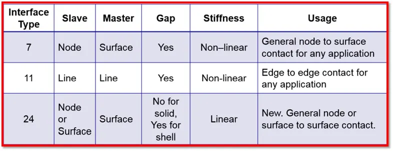
Figure 1-Commonly Used Interfaces Types for Impact Simulations.

1) Interface Penalty Method

2) TYPE7,Variable Stiffness,Node to Surface Contact.

3) TYPE11,Variable Stiffness,Edge to Edge Contact.

4) TYPE24,Linear Stiffness,Node to Surface and Surface to Surface Contact.

5) TYPE19,Combination of TYPE7 and TYPE11.

1) Interface Penalty Method :

The penalty method treats the behavior between slave nodes and master segments as springs that generate resistive forces as a function of penetration.

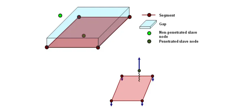
Figure 2-Penalty Method.

Here the interfaces are goverened by the penalty method.
When the parts come into contact,The slave node tries to penetrate the mid surface.
The solver introduces the 1D spring element once the slave node penetrates the gap.
The spring stiffness is automatically computed according to the material and property of both master segment and slave node.
If penetration is zero,the time step will be maximum.As the penetratiom goes on increasing,the time step goes on decreasing.
Time Step α">α�Stiffness.

Time Step for Contact Interfaces :

Nodal Time Step = Δt">ΔtΔ�≤">≤≤2MK">√2MK2��
Kinematic Time Step=Δt">ΔtΔ�≤">≤≤0.5(g-p)dpdt">0.5(g−p)dpdt0.5(�-�)��
Where dp/dt -Speed of the Sound Wave through the Material.
g-Gap
P-Penetration
Δt">ΔtΔ�-Time Step.
M-Mass
K-Stiffness

Interface Type 7 : Nodes to Surface Contact -

It is a general purpose interface and can simulate all types of impact between a
set of nodes and a master surface.
Non oriented and slave nodes can belong to the master surface,Hence auto impact possible.
Automatic node to surface contact interface using penalty method with variable stiffness.
A gap is defined around the master segment and the slave nodes.
The contact gap can be constant or variable.
Resistive forces are applied to keep slave nodes out of the contact gap.
Interface time step is computed to insure stability.

Important Interface Parameters :

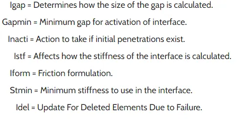
⋆">⋆⋆I_gap">I_gap�_��=Determines how the size of gap is calculated`

⋆">⋆⋆Gapmin">Gapmin��min=Minimum gap for activation of interface.

⋆">⋆⋆Inacti=Action to take if initial penetrations exist.

⋆">⋆⋆I_stf">I_stf�_��=Affects how the stiffness of the interface is calculated.

⋆">⋆⋆I_F">I_F�_�orm=Friction formulation.

⋆">⋆⋆Stmin">Stmin��min=Minimum stiffness to use in the interface.To avoid timestep error.

⋆">⋆⋆IDel">IDel��=What to do with slave nodes and master segments,if elements fails (deleted) that they are attached to or Update for Deleted Elements Due To Failure .

Gap Definitions :

`I`_gap=0	Constant Gap	The gap is defined by Gapmin">Gapmin��min and is constant for all the contacts.This is default value.
`I`_gap=1	Variable Gap	The gap varies according to the characteristics of the impacted master surface and impacting slave node.
`I`_gap=2	Variable Gap	Variable gap with gap scale factor.
`I`_gap=3	Variable Gap	Variable gap with gap scale factor and with mesh size correction.

Table-1

Inacti :

Inacti is nothing but Initial Penetration.
We will be giving this parameter to get rid off penetration in the model.

Initial Penetration :

Initial penetration result if a slave node is closer to the master segment than the calculated gap.
Initial repulsion forces give an error in the energy balance due to the interfaces work.
There are options in the solver to remove initial penetrations.
Inacti = 3 may create initial energy if the node belongs to a spring element.
Inacti = 6 is recommended instead of Inacti =5, in order to avoid high frequency effects into the interface.

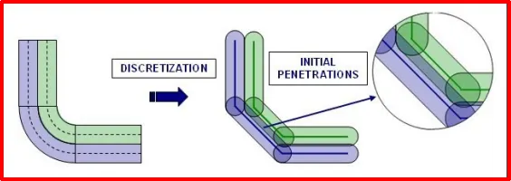
Figure 3-Initial Penetrations.

Initial Intersections :

Intersections result if slave nodes are past the master segment (shells or solids).
This condition can cause locking situations leading to computation failure.
If slave nodes lie on the master segment an ERROR will occur because of the Type 7 contact stiffness definition.

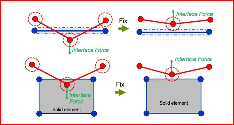
Figure 4-Initial Intersections.

Options for Removing Initial Penetrations :

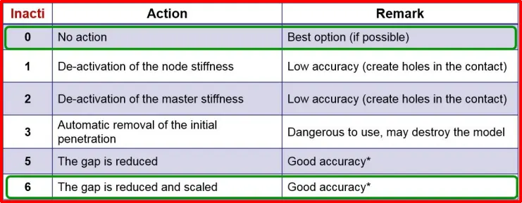
Figure 5-Options for Removing Initial Penetrations.

I_stfInitial Contact Stiffness :

We will be giving initial contact stiffness to get rid off penetration.
Like when two components are going to penetrate,To avoid this,we will be giving Initial Contact Stiffness.
For Example : If the soft component coming into contact with the hard component,the soft component will absorb the resisitive forces.So thats why the stiffnes of the soft component is considered.
Istf=4 is mostly recommended for the crash applications.

Iform (Sliding Force Computation ) :

The recommended parameter is Iform=2,Cause the sliding forces are computed using stiffness parameters.

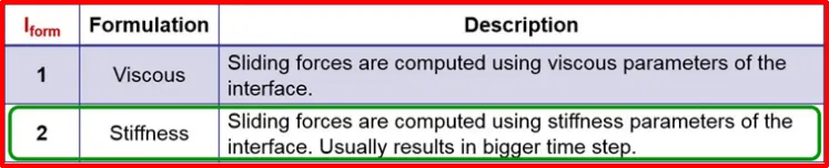
Figure 6-Iform Parameters.

Idel (Update for Deleted Elements Due To Failure) :

Idel indicates the update for deleted elements due to failure.

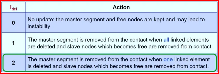
Figure 7-Idel Parameters.

Recommended Parameters for Crash Applications :

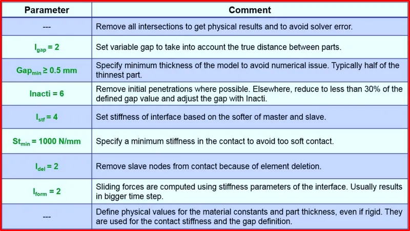
Figure 8-Recommended Parameters for Crash Applications.

Advantages and Disadvantages of Type 7 Contact :

Advantages :

Physically correct representation.
High accuracy for describing self-contact and buckling.
Best used with shells to shells or solids to shells.

Disadvantages :

Requires more stringent modeling practices.
Does not tolerate intersections (slave node passing master segment).
Time step may reduce due to increasing interface stiffness.

Interface Type 11 (Edge to Edge Contact) :

Type 11 is similar to the Type 7 Contact.
This interface simulates impact between edge to Edge or lines. A line can be a beam or truss element or a shell edge or spring elements. In association with interface TYPE7, interface TYPE11 solves the locking cases.
Defined by identifying master and slave lines (edges)
Impacts occur between a master and a slave line. A slave line can impact on one or more master lines. A line can belong to the master and the slave side. This allows self-impact.
Works similar to Type 7 in terms of Penalty formulation, Gap definition and search method.
Uses complicated mathematical algorithms; therefore, it is strongly advised to use it only when necessary. A huge interface TYPE11 can slow down the computation.

Procedure :

1) Mesh the Bumper assembly with 6mm size.

First import the bumper assembly into the GUI which is shown in below image.

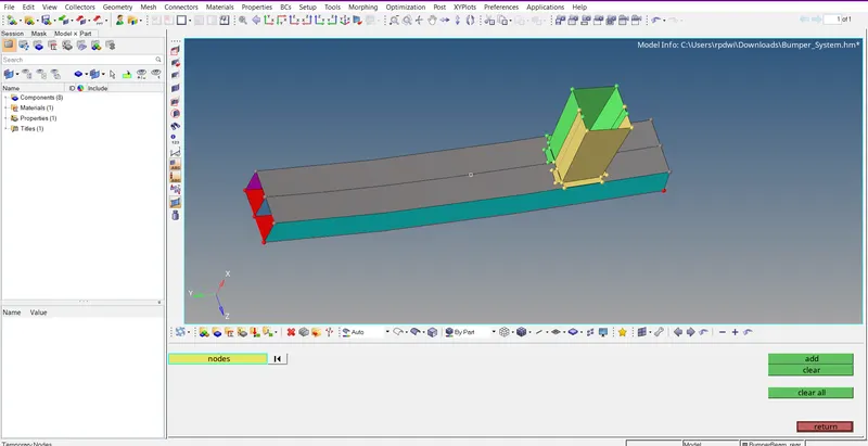
Then view the component in topo mode which is shown in the below image.
Delete temp node by using (Geom>Temp Node>Clear All).

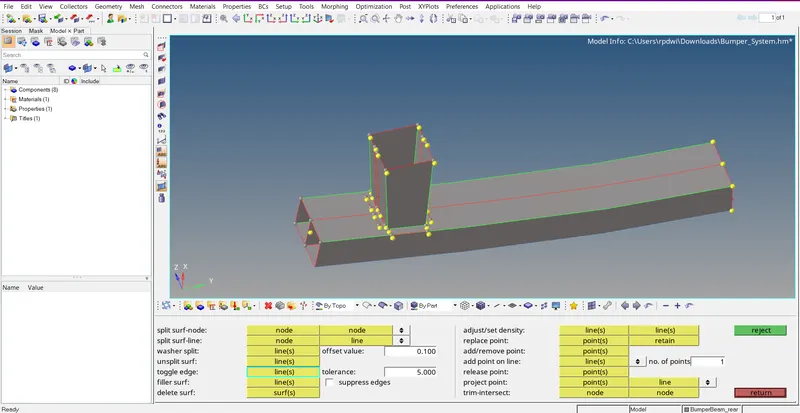
As shown above image below part having one free edge to remove this type of error by using (Surface edit>Extand>Select line>Select target surface>Extand)
Free Edge rem0oved and red line turn into yellow line.

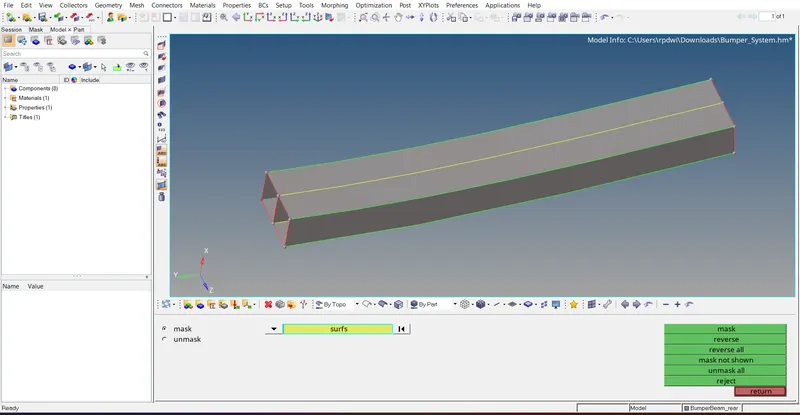
Here surface is not in proper or not connected watch other to remove use Geom>replace point or tongle option.

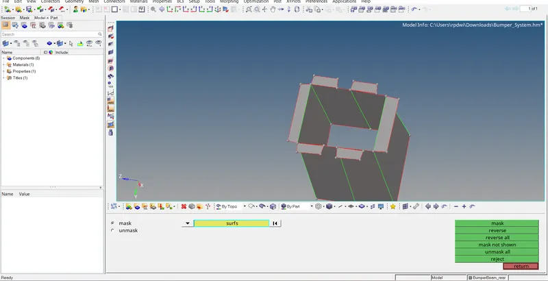
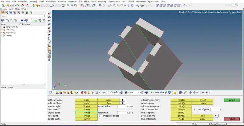
Finally got the result as shown below image.

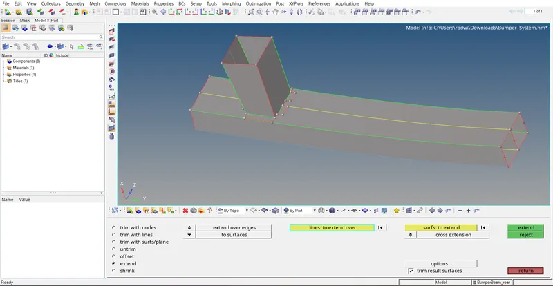
Now start meshing by using (F12 or 2d>Automesh>Traget element size As 6>Mesh )
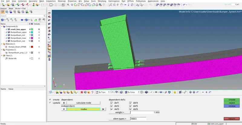
Once the mashing did give a connection to the connected part by RBE3 by using(2d>Connector>rbe3>select node by path>Create)

Import the Starter File into the Solver Deck Radioss :

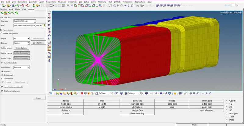
While opening hypermesh software,A user profile window will pop up,Switch to the radioss user profile as shown in below Figure 26 and start importing the model into the solver deck.

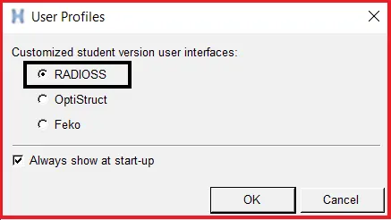
Now after switch the user profile to radioss,import the model (starter file) into the radioss solver deck.
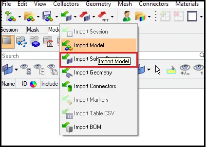
To import the model,Go to Standard Panel >> Import >> Import Solver Deck.

To switch to shaded mode,Go to Visualization Tab >> Shaded Elements and Mesh Lines.

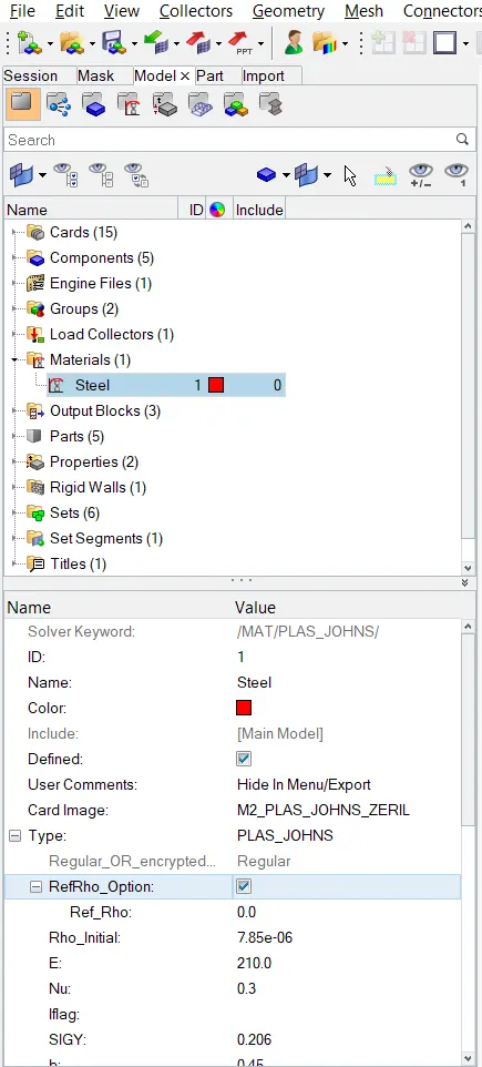
importent interface parameters

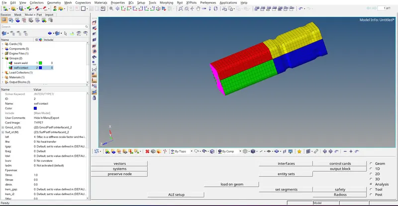
Case-1 Run the Crash Tube Model as it is default :

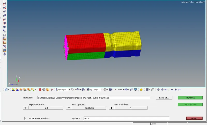
Now run the simulation, To run the simulation, Go to Analysis Panel.
Go to Analysis Panel >Radioss >Select the Input File > Save it in Different Folder and Rename it as Case-1 > Run.
Check the Include Connectors, If there are any connectors in the model, The connectors will also be taken into account.
Type -NT 4 in the options tab, This will make the simulation faster.
Where NT indicates No of threads,4 indicates assigning the task to 4 cores in the system.
Here save the input file in a different folder, and rename it as case-1 which
- Now run the solver by hitting on radios.

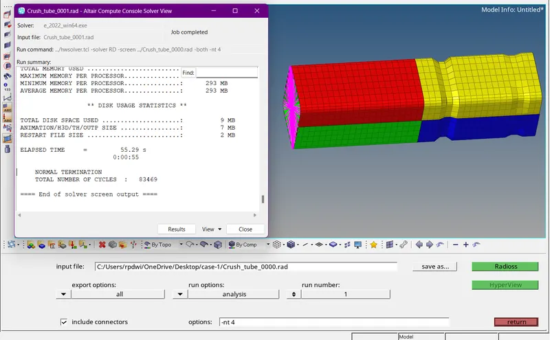
After completing the simulation,the radioss will pop up a solver window stating Radioss Job Completed which indicates the simulation has been completed

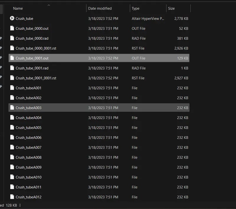
After running the simulation,The animation files will be generated where we specified a location to store the files

Now go and open the 00001.out file with notepad.
The obtained values for Energy Error,Mass Error,Internal Energy Error,Kinetic Energy Error and Contact Energy Error

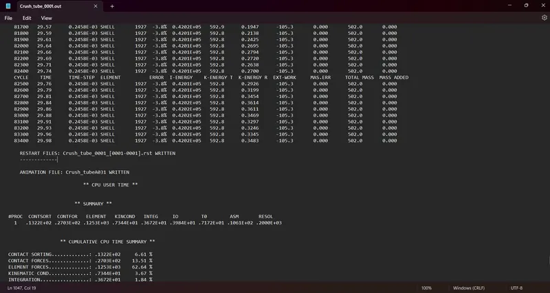
Energy Error-(-3.8%)

Internal Energy-0.4202E+05

Kinetic Energy-592.8

External Work-(-105.3)

Mass Error-0

Total No of Cycles-83400

Postprocessing of Case-1

1) Review the Simulation using -HyperView.

2) Plot the graphs using -Hypergraph 2D.

1) Review the Simulation using HyperView :

- After analysis go for the hyper view to run the animation file.
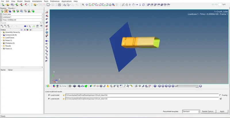
Import the animation file .h3d into the hyperview.
After loading the model into hyperview,It will be represented as shown in below.

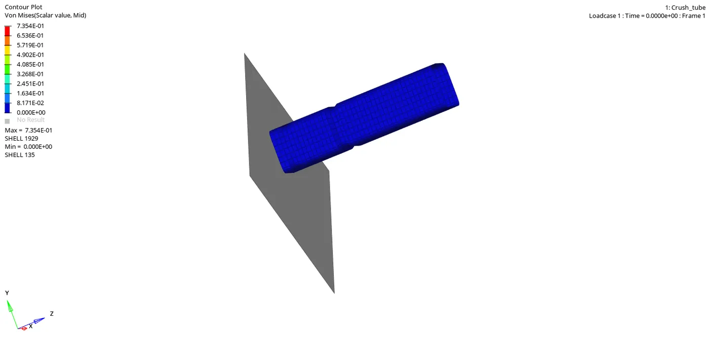
Now switch to the Von Misses Stress in result type and select the component,select the averaging method as simple and then click apply as shown in below image.

After applying ,Run the Simulation,The Simulation animation is shown in below image.

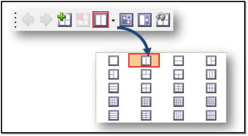
The pages can be split into 2 so that perform the other operations in to account. Use the expand and reduce the window.

2) Plot the graphs using -Hypergraph 2D.

Now plot the graphs using Hypergraph 2D,We are plotting the graphs to see what is happening in the rail component.
Hypergraph 2D is a powerful data analysis and plotting tool with interfaces to many popular file formats.
It is sophisicated math engine capable of processing even the most complex mathematical expressions.
Hypergraph 2D combines these features with high quality presentation output and customization capabilities to create a complete data analysis system for any organization.

Here switch to the Hypergraph 2D to plot the graphs.
To switch,Go to Client Selector >> Choose the Hypergraph 2D as shown in above

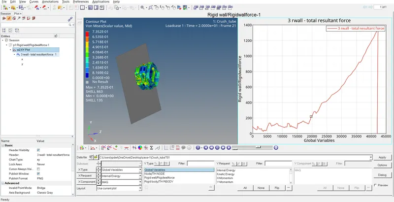
Rigid Wall Forces :

Here the rigid wall forces starts from origin,Cause initially there is no contact between the crash tube and rigid wall.
And it goes on increasing,cause the elements are getting deformed and the rigid wall forces suddenly reaches peak,cause the entire crash tube collides with the rigid wall.
And again its decreasing,cause after the collision,the entire component will be at rest,So its decreasing.

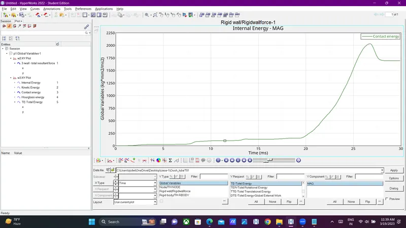
Contact Energy:

Here the contact energy starts from origin,Cause the crash tube component is in intial condition.
Intially there is no contact between the crash tube component and rigid wall.
There is also no deformation intially,But when the component goes and hits on the rigid wall,The contact energy starts increasing.
When the deformation or displacement happens to the component,the contact energy increases,cause the crash tube comes into the contact to the rigid wall.So the contact energy goes on increasing.

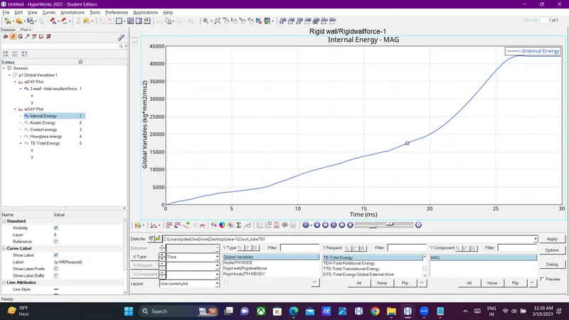
Internal Energy :

The formula for Internal Energy is I.E = Q±">±±W.
Here the heat is neglected,Cause there is no heat transfer,We will be having only workdone.
W=FxD
F=ma
Here the internal energy is in Zero,Because there is no deformation initially,So the internal energy is in Zero and starts from Zero and goes on increasing.
The internal energy increases because the deformation is happening,there is a displacement,So the internal energy increases,when the displacement or deformation occurs.

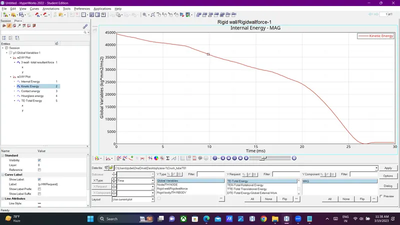
Kinetic Energy :

given for the component.
And it goes on decreasing,cause the deformation is happening to the crash tube,so the kinetic energy is decreasing.

Total Energy:

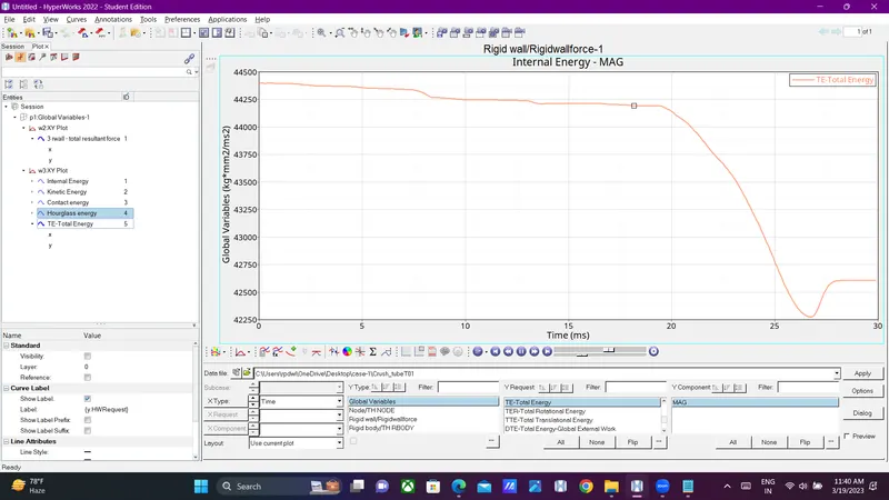
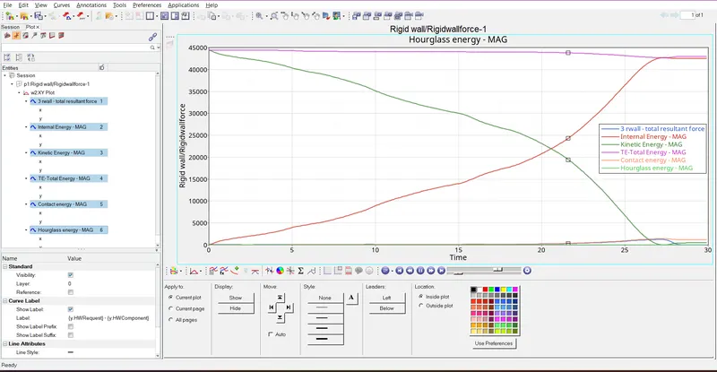
Total Energy is sum of Kinetic Energy+Contact Energy+Hourglass Energy + Internal Energy.
Here total energy starts from higher value,In starting itself its increasing,Why because the total energy is sum of Kinetic Energy+Contact Energy+Hourglass Energy + Internal Energy.
All energies are in initial condition except kinetic energy,So kinetic energy is only there
Total Energy=Kinetic Energy+0+0+0.
Kinetic enrgy is directly proprtional to the total energy.
So the total energy is increasing in the beginning.
And its slightly decreasing,Due to -3.8% of energy error,the total energy is decreasing.

Hourglass Energy:

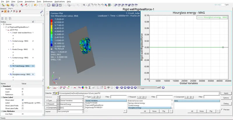
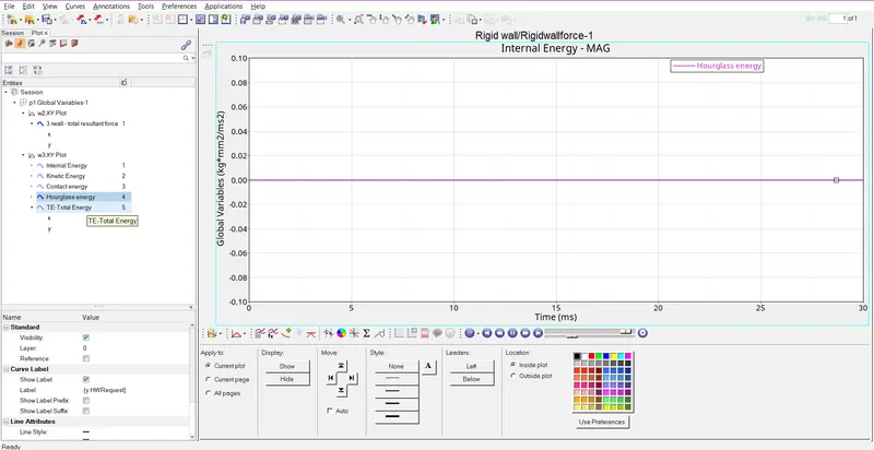
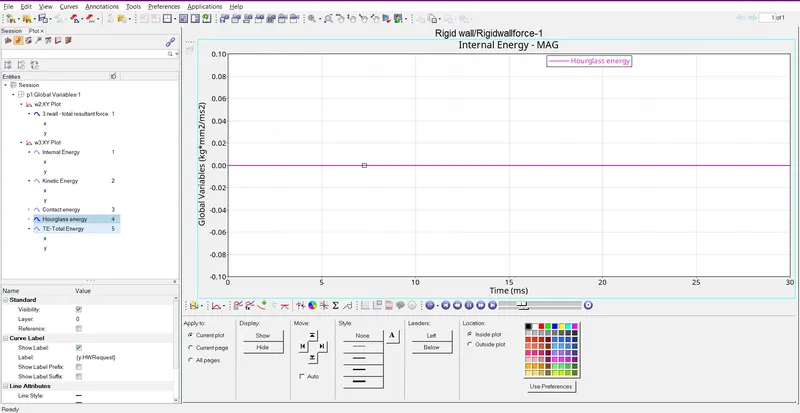
Here the hourglass energy is constant,Because the recommended parameter Ishell=24 has been assigned to the property card,So the hourglass energy is constant.

All Energies :

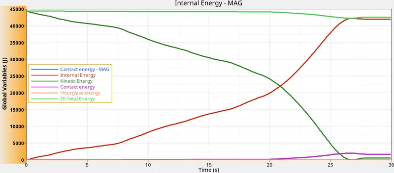
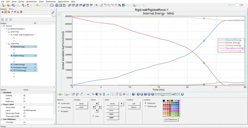
The obtained internal energy graph appears as soon The internal energy increases to the peak value at the end of the collision. And becomes constant. The Kinetic energy which is having higher value at the start of the simulation decreases as the simulation progresses with time and gets converted to internal energy, thus internal energy increases with time. The Total energy in the system is almost constant where the slight decrease is due to the energy error which is caused due to the resistive forces between master segment and slave nodes.

Case-2 Change the Inacti=6 and run :

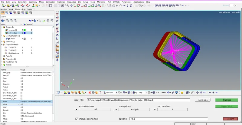
Here change the parameter value as Incti=6,Keep the remaining parameters as it is default.
When we change the Inacti Parameter=6,It will remove the penetration,the penetration won't happen between the slave and master node.
It will reduce the gap and adjust the gap.Like the gap will be reduced and scaled.The Iancti value is changed which is shown in below image.

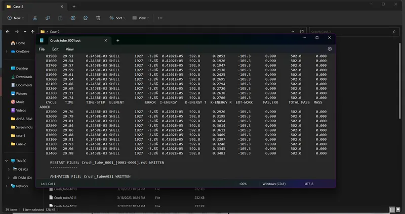
Now go and open the 00001.out file with notepad.
The obtained values for Energy Error,Mass Error,Internal Energy Error,Kinetic Energy Error and Contact Energy Error has been shown in below image.

1) Review the Simulation using -HyperView.

After completion of running the simulation,Switch to the hyperview.
Open the appropriate .h3d file to review the simulation.
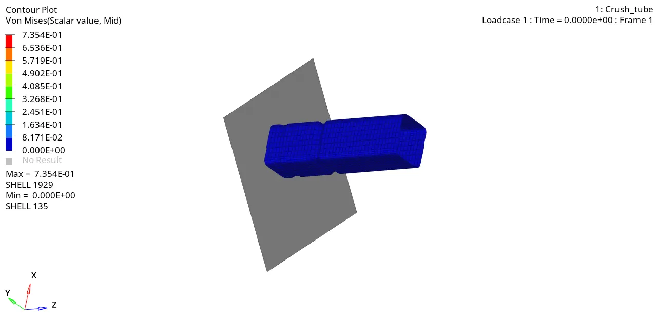
The .h3d file is loaded and it is shown in below simulation image.
Here the stess generated for this case is 0.73 Mpa.The behaviour is same similar to the previous case 1.

2) Plot the graphs using-Hypergraph 2D.

Now switch to the Hypergraph 2D and plot the graphs.
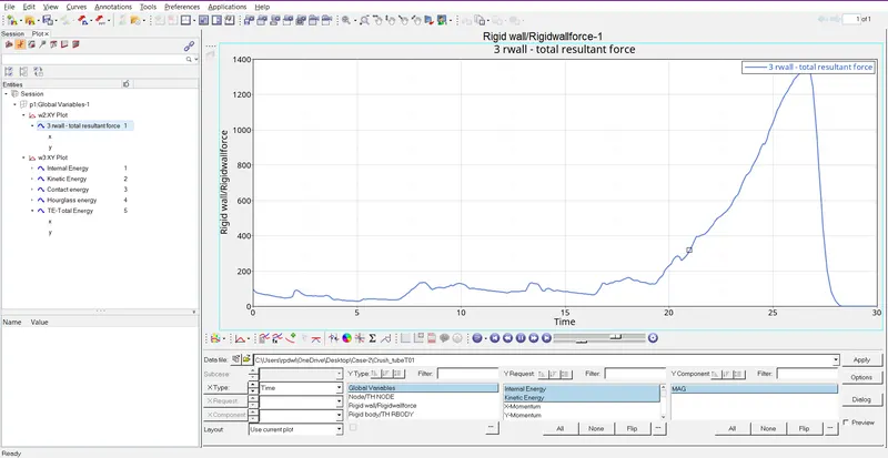
The rigid wall forces graph is plotted which is shown in below

Rigid Wall Forces :

The obtained graph for rigid wall forces is shown in below image. Here The rigid wall forces is similar to the previous case 1.

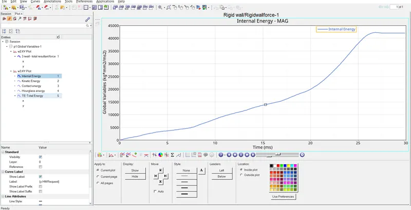
Internal Energy :

The obtained graph for internal energy is shown in below image.Here aslo internal energy is similar to the previous case 1.

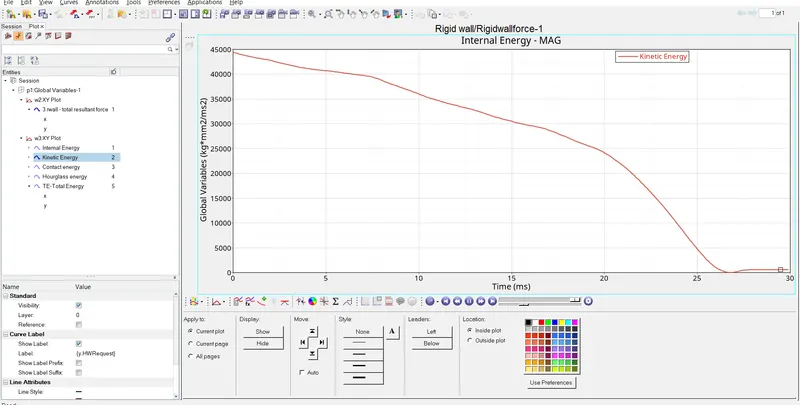
Kinetic Energy :

The obtained graph for kinetic energy is shown in below image.Here aslo kinetic energy is similar to the previous case 1.

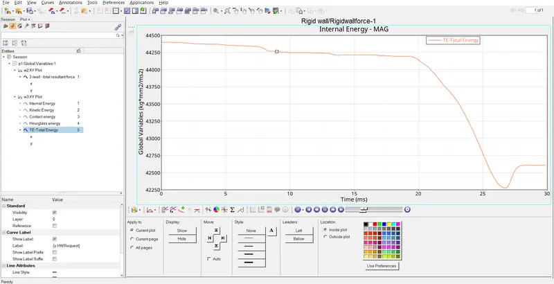
Total Energy :

The obtained graph for total energy is shown in below image.Here aslo total energy is similar to the previous case 1.

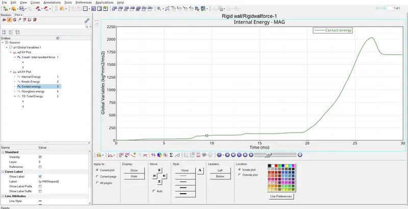
Contact Energy :

The obtained graph for contact energy is shown in below image.Here aslo contact energy is similar to the previous case 1.

Hourglass Energy :

Here the hourglass energy is constant, Because the recommended parameter Ishell=24 has been assigned to the property card, So the hourglass energy is constant.

[Note: Hourglass Energy is constant for all the 6 cases, Because the recommended parameter Ishell=24 has been assigned to the property card, So the hourglass energy is constant.]

All Energies :

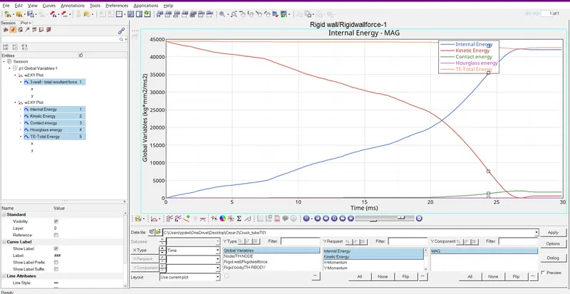
Case-3 Create the type 11 contact and run :

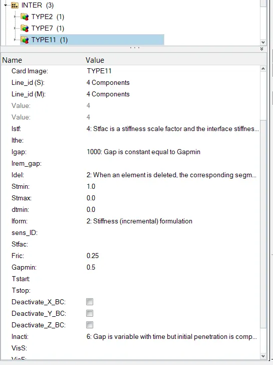
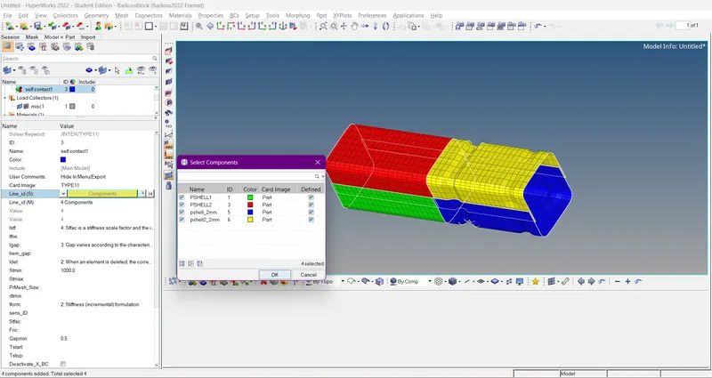
In this case, the new contact named "Type 11". In this contact, some parameters are to be entered, as shown in In order to get, the better results.

1) Review the Simulation using -HyperView.

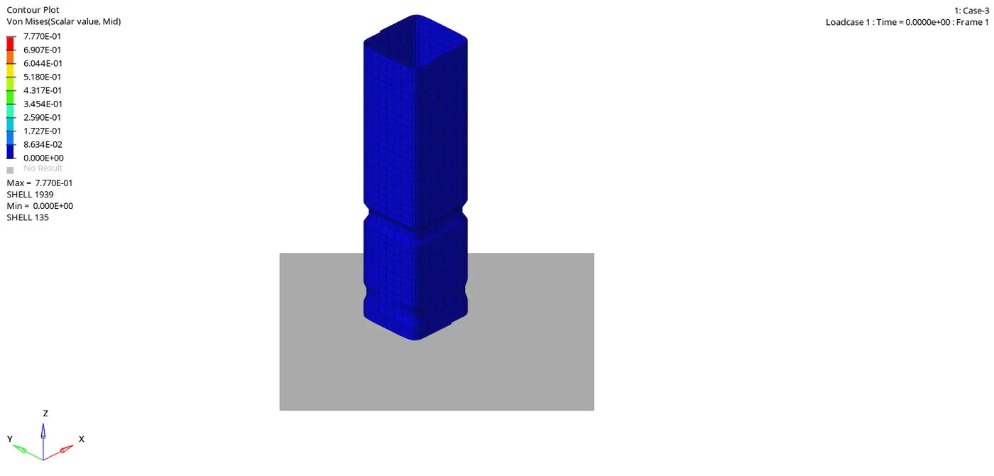
Now run the simulation,After running the simulation,Switch to the Hyperview and load the .H3D file to view the results of the simulation which are shown in below sim.image

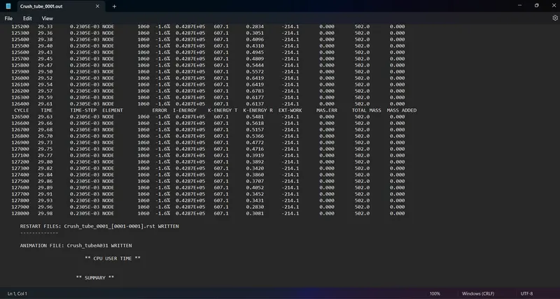
Now go and open the 00001.out file with notepad.
The obtained values for Energy Error,Mass Error,Internal Energy Error,Kinetic Energy Error and Contact Energy Error has been shown in below image.

2) Plot the graphs using -Hypergraph 2D.

Rigid Wall Forces :

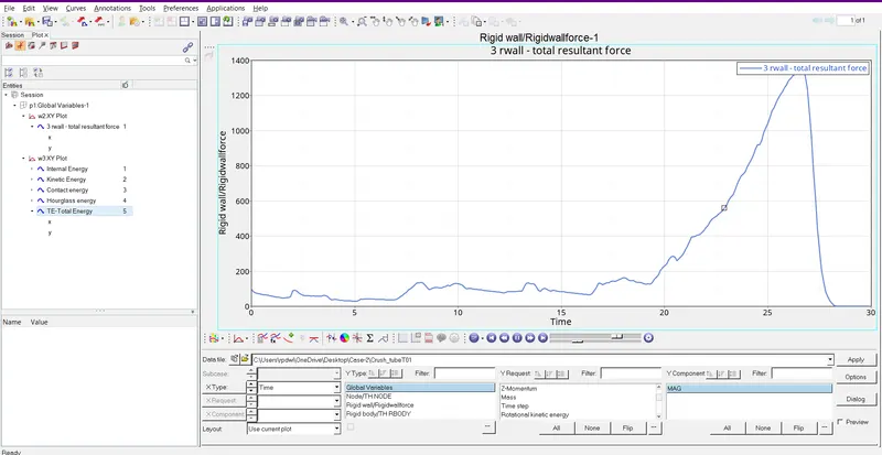
The graph obtained for the rigid wall forces is shown the below image.
Here the rigid wall forces are increased when compared to the previous case.It is increased between the range of (1400-1600).
They are increased cause the type 11 contact is also defined with the type 7 contact,so they are increased.

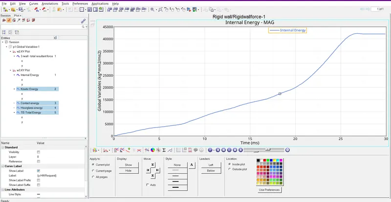
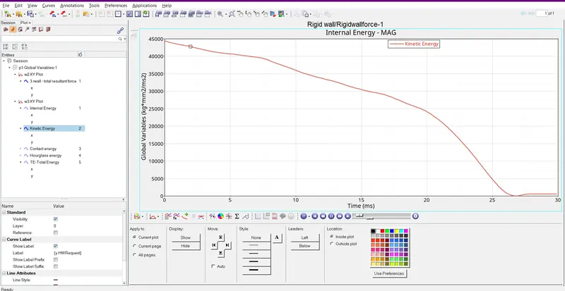
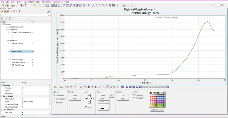
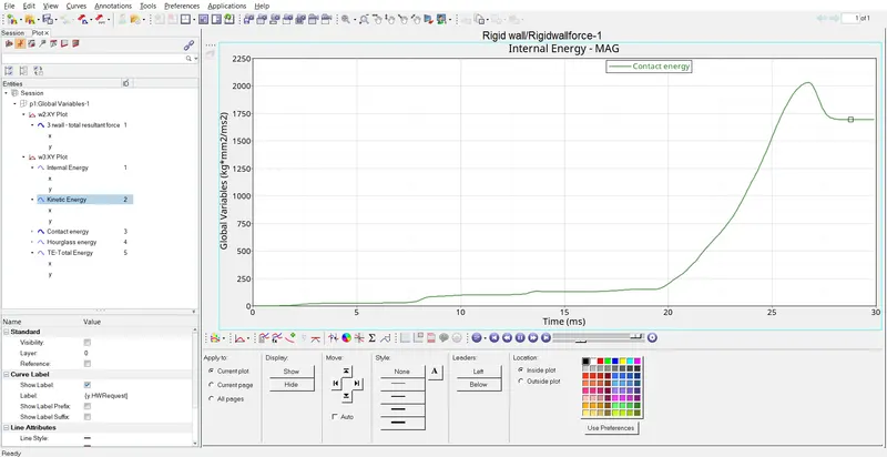
Here the Kinetic, Internal, Contact, Internal, and Hourglass Energy are similar to the previous case.
The graphs plotted for Kinetic, Internal, Contact, Internal, and Hourglass Energy are shown below Figure 80.

Kinetic Energy:

Contact Energy:

Hourglass:

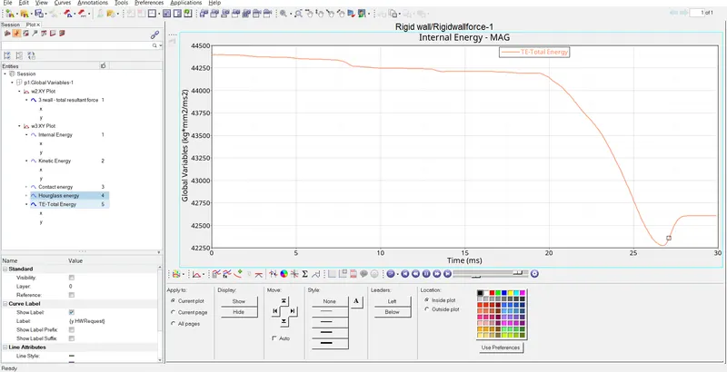
Total Energy:

All energy's:

Case 4-Remove both notches and remove boundary condition on rigid body node then run :

Here in this case,We have to remove the notches and boundary conditions as per the question.
To remove the notches,use align node tool and align them properly to remove the notches.
To Align,Go to Geometry >> Node Edit >> Node 1,2,3 >> Align Node.
The notches have been removed for this case,which is shown in below Figure 88.

by the removing notche's by using (Geom>Node edit>Align Node>select 1st node>2nd node>node>Align)

in this case we remove both notch's and remove Boundry condition (BCS) or give type of contact Type11 and given main [[parameter in type 11 contact after all these changes run the analysis

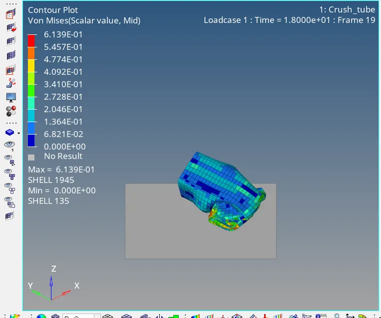
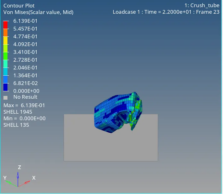
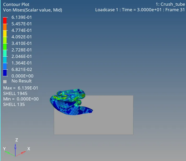
The energy error this time was just 0.1 %. A reduction can be there due to the free movement of the crush tube upon impact as the restriction on the rigid body was removed.

The crush tube can be seen bouncing off at the end of buckling, this is the effect of constraint removal from the independent node of the rigid body. Next, we need to examine various plots obtained using the hypergraph.

2) Plot the graphs using -Hypergraph 2D.

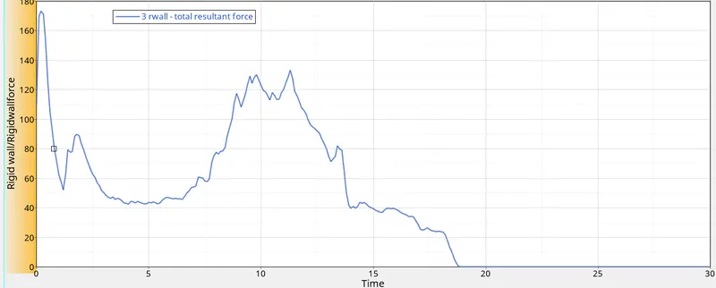
Rigid Wall Forces :

AS below graph rigid wall force start from 150 because till time there no force applied or there is no contact with rigid wall connectoin.
after that crush tube getting deformation start and graps goes up 165.
than part deforming and graps decreasing because there no notch present.
similarly part behaving deform because no boundary condition and than crash tube bounced and found straight line.

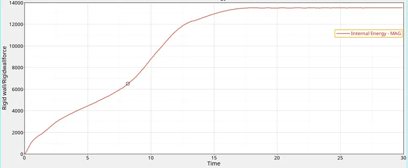
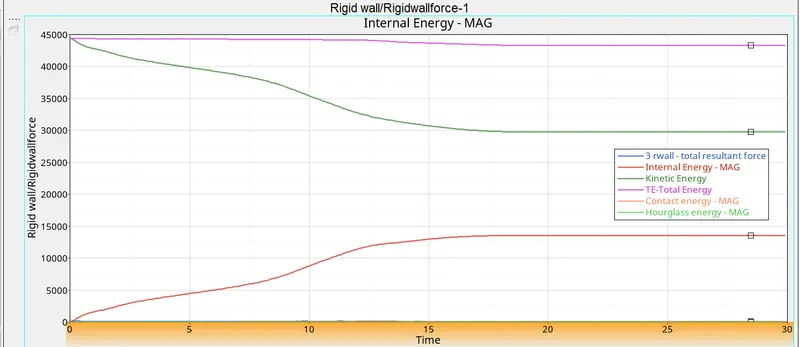
Internal Energy.

The obtained graph for internal energy is shown in below image.Here aslo internal energy is similar to the previous case

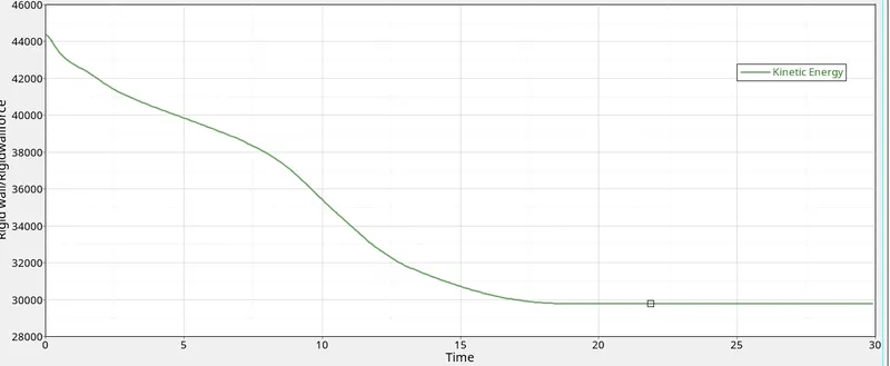
Kinetic Energy :

The obtained graph for the Kinetic Energy is shown in below image.
It is similar to the previous case.

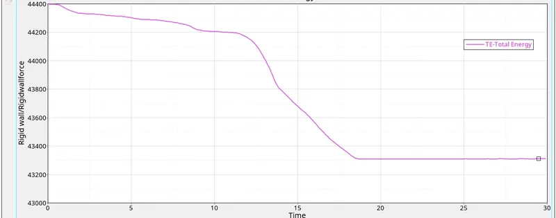
Total Energy :

The obtained graph for the Total Energy is shown in below image.,
It is similar to the previous case.

Case-5 Create a new notch in the middle ,select the whole section and run :

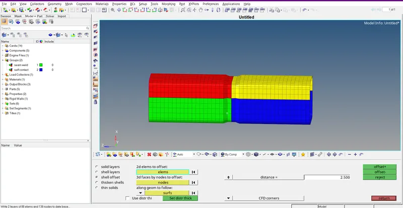
Here for this case,Create notches in the middle by using element offset.
To create notches in the middle,Go to 2D panel >> Element Offset >> Select Elements >> Distance=2.5>> Offset+.

1) Review the Simulation using -HyperView.

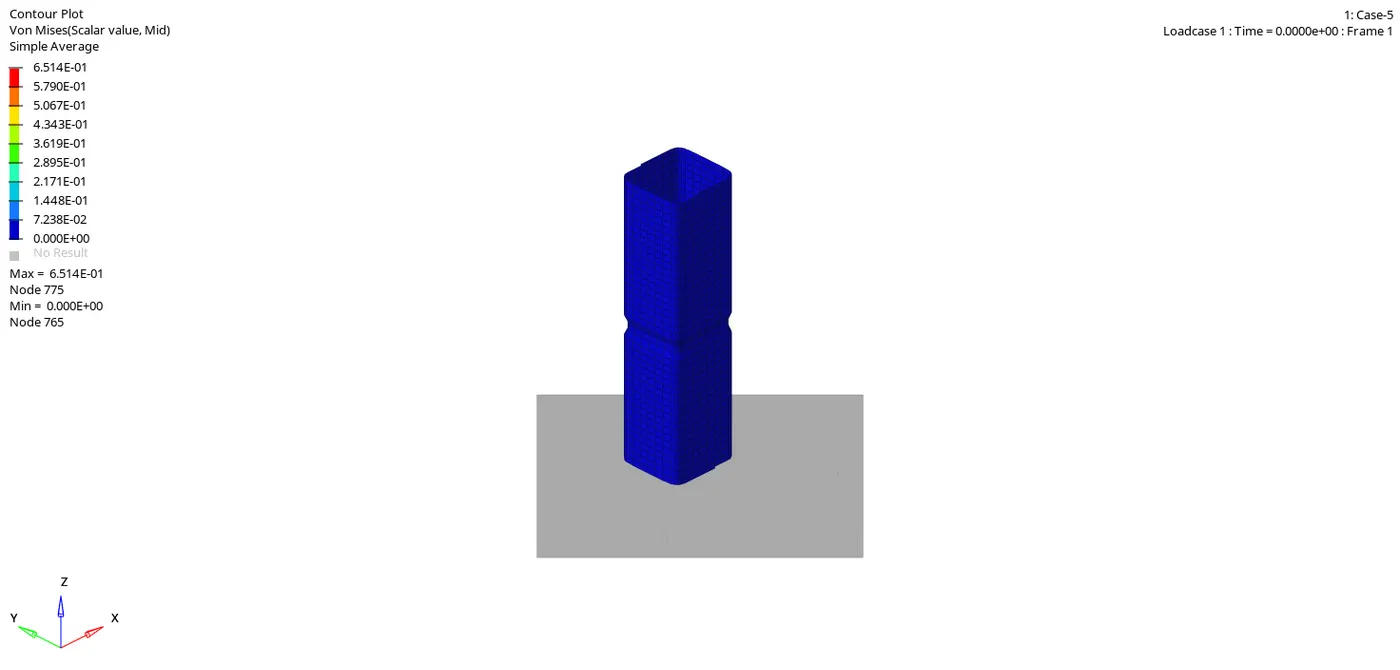
Now run the simulation,After running the simulation,Switch to the Hyperview and load the .H3D file to view the results of simulation which is shown in below image.
Here the buckling is happening,Where the notches exsist.

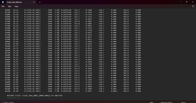
Now go and open the 00001.out file with notepad.
The obtained values for Energy Error,Mass Error,Internal Energy Error,Kinetic Energy Error and Contact Energy Error has been shown in below image.

2) Plot the graphs using -Hypergraph 2D.

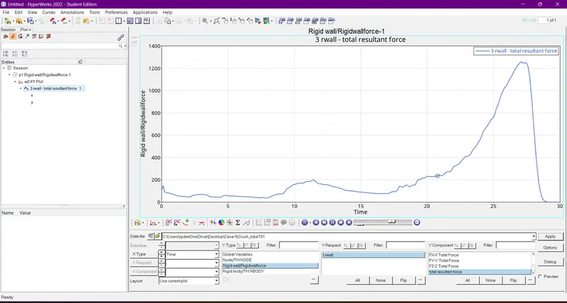
Rigid Wall Forces :

The obtained graph for rigid wall forces is shown in below image
Here the rigid wall froces are similar to the previous case,But the buckling is happeneing where the notches exsist in the crash tube.

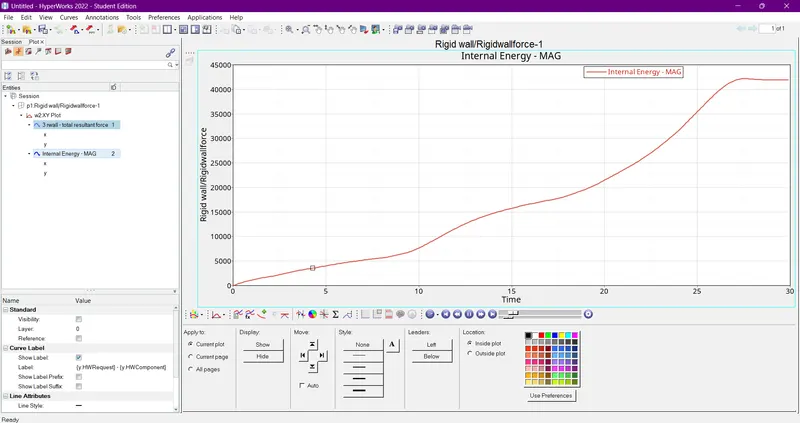
Internal Energy :

The obtained graph for the Internal Energy is shown in below image.
It is similar to the previous case.

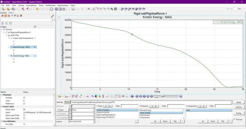
Kinetic Energy :

The obtained graph for the Kinetic Energy is shown in below image.
It is similar to the previous case.

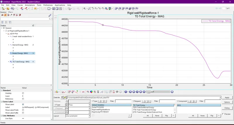
Total Energy :

The obtained graph for the Total Energy is shown in below image.
It is similar to the previous case.

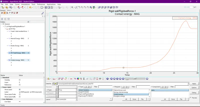
The obtained graph for the contact forces is shown in below Figure 105.
Here the contact Energy are also some what similar to the previous cases.

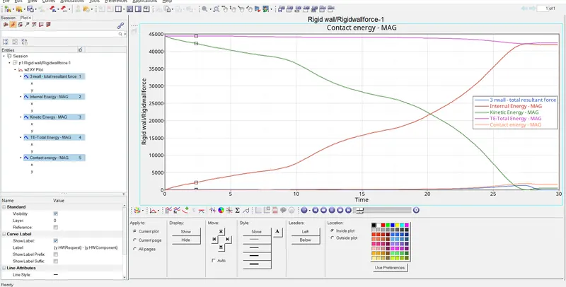
Case-6 Create a new notch with nodes only from opposing 2 faces and run :

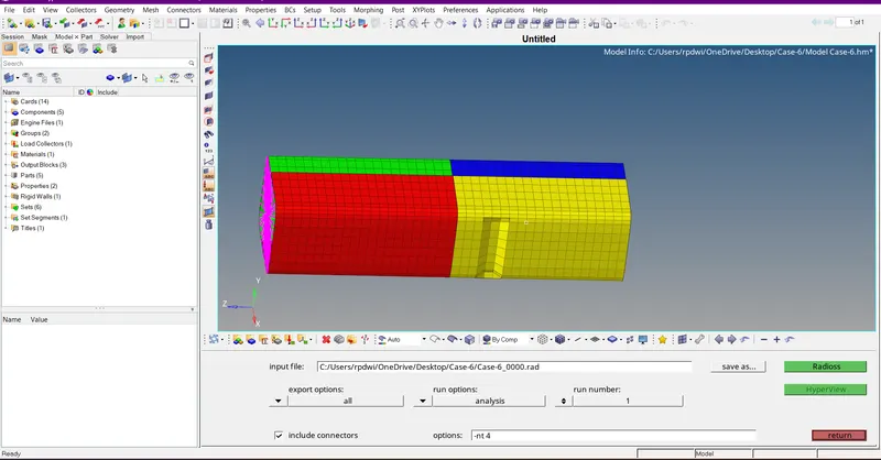
Here for this case create a notch in the two opposite faces and run the simulation.
The notches created in the two opposite faces is shown in below image.

1) Review the Simulation using -HyperView.

Now run the simulation,After running the simulation,Switch to the Hyperview and load the .H3D file to view the results of simulation which is shown in below Image.
Here also the buckling is happening,Where the notches exsist.

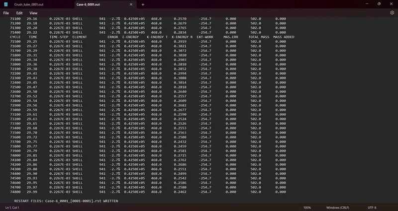
Now go and open the 00001.out the file with notepad.
The obtained values for Energy Error, Mass Error, Internal Energy Error, Kinetic Energy Error, and Contact Energy Error have been shown in below image.

2) Plot the graphs using -Hypergraph 2D.

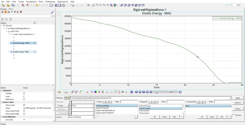
Kinetic Energy :

The obtained graph for the Kinetic Energy is shown in below image
It is similar to the previous case.

Internal Energy :

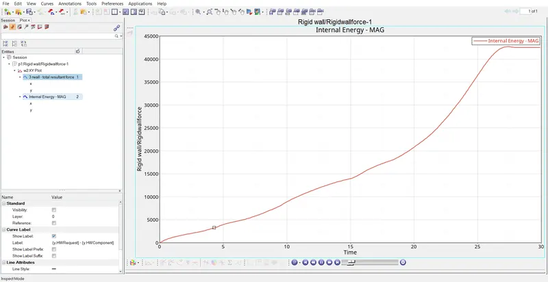
The obtained graph for the Internal Energy is shown in below image.
It is similar to the previous case

Rigid Wall Forces :

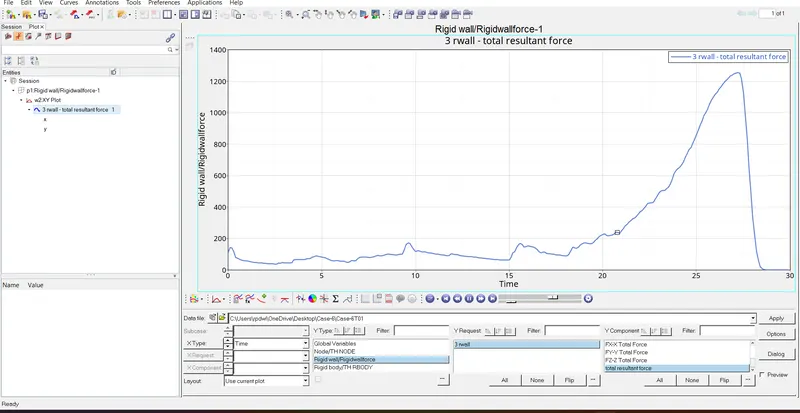
The obtained graph for rigid wall forces is shown in below image.
Here the rigid wall forces are similar to the previous case,But the buckling is happeneing where the notches have been created in the crash tube.

All Energies :

Comparison of all the Cases -

Cases	Energy Error	Internal Energy	Kinetic Energy	External Work	Mass Error	Elapsed Time	Total Number of Cycles	Interface Type	Changes in Model
Case-1	-3.8%	0.4202E+05	592.6	-105.2	0.000	373.09 s	83496	TYPE 7	No Change.
Case-2	-3.8%	0.4202E+05	592.6	-105.2	0.000	197.72 s	83496	TYPE 7	Changed into Inacti=6.
Case-3	-1.6%	0.4285E+05	610.7	-214.7	0.000	1313.44 s	127876	TYPE 11 and TYPE 7	Changed into Recommended Parameters.
Case-4	-3.2%	0.4224E+05	569.7	-172.9	0.000	487.83 s	75741	TYPE 11 and TYPE 7	Removed Notches and Boundary Conditions.
Case-5	-3.0%	0.4217E+05	672.7	-244.9	0.000	572.15 s	92781	TYPE 11 and TYPE 7	Created Notches in the Middle.
Case-6	-3.1%	0.4214E+05	532.6	-365.6	0.000	526.16 s	97519	TYPE 11 and TYPE 7	Created Notches in the Opposite Faces Only.

Table-1

Result :

Hence the simulation for all the cases were carried out with different parameters.
Hence the simulation for all the cases were runned successfully.
Hence the simulation for all the cases were reviewed by hyperview.
Hence the graphs were plotted for all the cases successfully.
Hence meshed the bumper component with 6 mm size.
Atlast,Compared all the results for those cases.

Conclusion and Learning Outcome :

In this challenge,I came to know bout
The types of interfaces and their applications.
The effect of notches in the model.
The penetration causes.
The diferent parameters for the interfaces.
The elements deform during the interface.

Assignment 5-RADIOSS Interfaces & Study of Effect of Notches Challenge

Assignment 5-RADIOSS Interfaces & Study of Effect of Notches Challenge

Ship work like this
in your own course.

Talk to a career counsellor

Assignment 5-RADIOSS Interfaces & Study of Effect of Notches Challenge

Ship work like thisin your own course.

Talk to a career counsellor

Ship work like this
in your own course.