Assignment 5-RADIOSS Interfaces & Study of Effect of Notches Challenge

Objective:

1. To mesh the given bumper assembly with a mesh size of 6mm

2. To carry out simulations on the given crush tube model, so as to compare results as per the following requirements for each case:

1. Run the crash tube model as it is.
2. Change the Inacti=6 and run.
3. Create the type 11 contact and run.
4. Remove both notches and remove boundary condition on rigid body node then run.
5. Create a new notch in the middle, select the whole section and run.
6. Create a new notch with nodes only from opposing 2 faces and run.

PROCEDURES
Meshing the bumper assembly

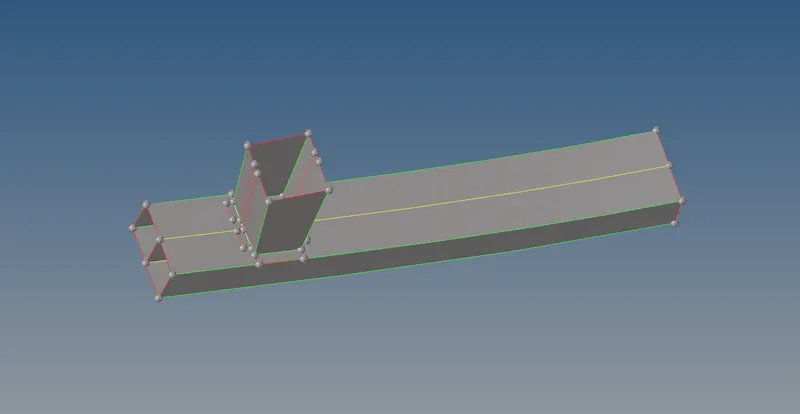
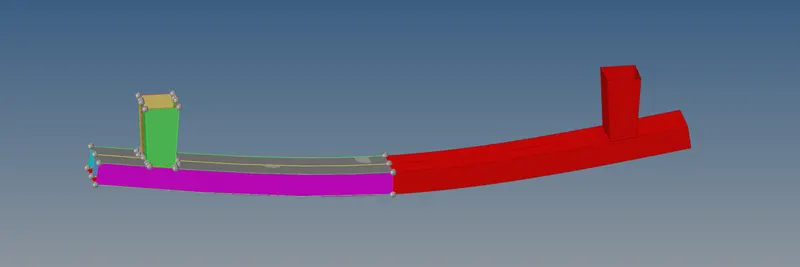
1. After importing the bumper assembly on Hypermesh, the first step is to carry out geometry cleanup using the various quick edit tools (Geometry > Quick Edit). Also, Geometry > Surface Edit > Extend is used to ensure the panel in the centre intersects the outer panels to create the non-manifold edge that is yellow in colour. After clean up is carried out, it should look like this,

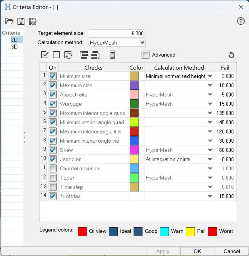
2. After cleaning up, we can set it up for meshing. We can assign the mesh quality criteria via Preferences > Criteria File Settings and assign the values as follows:

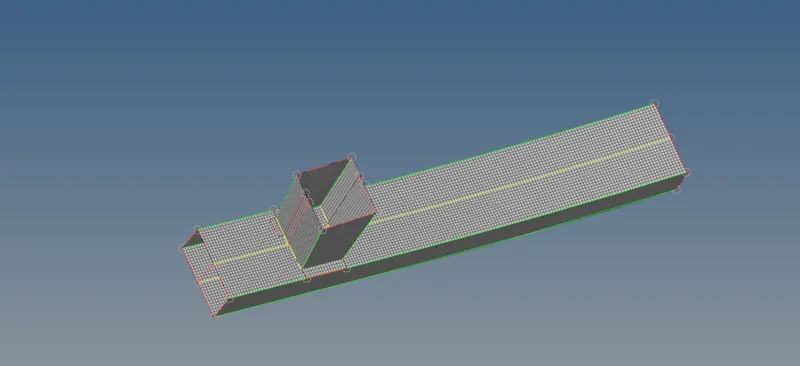
3.We can then move onto meshing via 2D > Automesh in the bottom panel. Since all the components have rectangular faces, we can directly mesh each face without having to split it up to avoid trias. With the mesh size set as 6mm in the automesh menu, this is the meshed assembly.

4. Since this is just one side of the bumper, we can use the reflect tool to replicate the other half of it. Reflect tool can be accessed via Tools > Reflect. Selecting the axis along which it is to be reflected, and the base point, along with all the elements duplicated, we can go ahead and click 'reflect' to generate the other half.

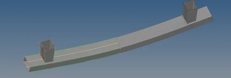
After this, we need to equivalence the mesh in the centre since they won't be connected. This is done using Tools > Edges. We can select all the elements and adjust the tolerance to find regions that lack equivalency. After highlighting them using 'preview equivalency', we click 'equivalence' to finish up.

Simulations:

case 1: Run the crash tube model as it is.

• In this case, we need to run the simulation on the crush tube as is. we will be discussing the Type 7 interface when inacti is set to 0 (Default).

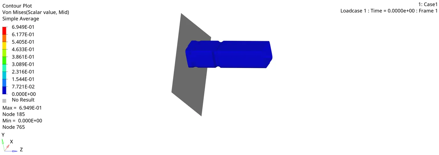
• From the animation, we can clearly see that the deformation taking place at the middle notch first due to applied velocity
• Once mid notch deforms the next deformation occurs in the second notch which is near to rigid wall this is because the thickness is less at bottom
• Here notch elements deforming inside and the rest flat elements are coming outside. This region does not require more force to deform the elements
• It is evident that the presence of notch leads to stress concentration in those regions. So, the buckling occurs first. This will happen in all the cases which have notches.
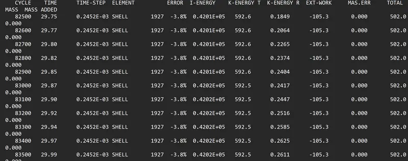
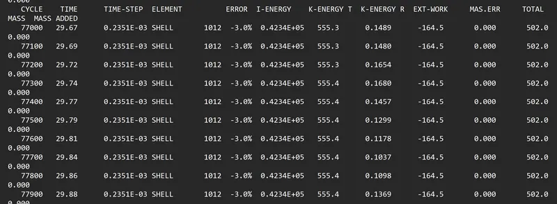
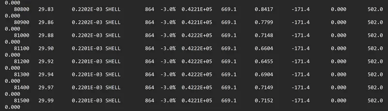
• As we can see, the energy error is -3.8%. It is acceptable since it is below -15%. In addition to that, there is no mass error (0%).

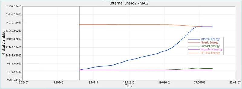
• Internal energy keeps increasing because the tube continuously absorbs energy while crashing onto the rigid wall, which results in deformation. You can see at last when the deformation completes, the internal energy goes constant.
• Kinetic energy keeps decreasing due to the initial velocity on the tube. The curve starts from high values and decreasing to low due to the deformation. There is a slight increase afterward due to rebound after deformation.
• Contact energy is a type of energy that is created when one element contacts neighboring elements. The opposing force created by the element is called contact energy. There is no contact in the initial stage, so that’s why the graph goes constant. After some time, the graphs slightly increase due to the buckling of elements. While the entire tube pressing on the rigid wall, the buckled elements are forced into contact.
• Total energy decreases at some point due to increasing of contact energy at the same time. so, the contact energy affects the total energy.
• Hourglass energy is constant due to the presence of recommended properties.
• Now next step is to plot the rigid wall resultant force graph for case 1 simulation, so select variable as rigid wall and parameter as resultant force and apply to plot the graph.

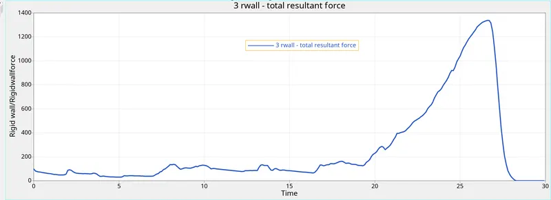
• It is evident that the rigid wall experiences some forces suddenly, due to the crush tube crash over the rigid wall and absorb the energy from crush tube. after the deformation completes, the rigid wall force is decreased immediately due to the energy transferred completely.

• The self-contact force from the TH inter card helps identify the forces due to the Type 7 contact formulation.
• The max self-contact force is 133.18N, which occurs at the end of the simulation, this is the point where a maximum number of master and slave segments are in contact with each other.

CASE 2: Change the Inacti=6 and run.

In this case, we shall be using Hypercrash as well. So, continuing past the second step outlined in the procedure, we can import the given crush tube model using File > Import.

After importing, we can go ahead and switch to the model browser tab. After that, we can move on to contact interface > self contact. We can then right-click 'self contact' and select the option 'see in panel'.

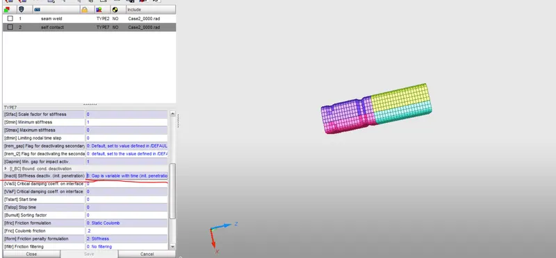
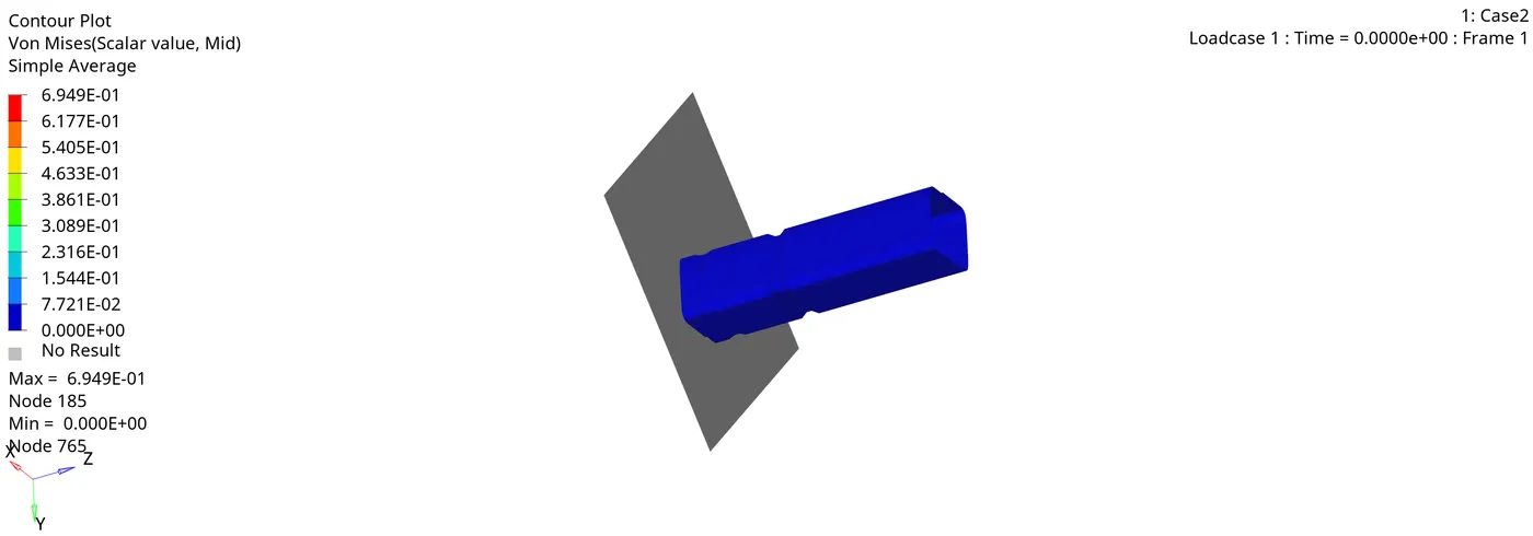
• There isn't any discernible difference between case 1 and case 2 animations, they're both very similar. Even though the Inacti parameter was changed, it didn’t have any effect on the simulation as there was no initial penetration to manage in the first place.
• Next, we can look at the output file which is shown below:

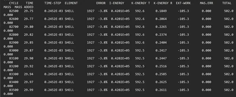
• As we can see, the values are the same as in case 1. The energy error is the same -3.8% (also the same mass error of 0%). Moving on to the plots

• There isn't much difference in the graphs, they are exact copies as that of case 1. The only thing we have learned from the energy plot is that there is no initial penetration since there is no difference between case 1 and case 2 energy plots (since the simulation was tweaked to detect such penetrations through the inacti function). If any initial penetrations existed, internal energy would start from a non-zero value.
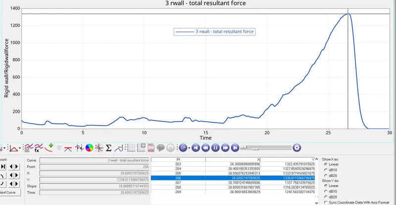
• RWall forces also exhibit the same characteristics as of case 1 as shown below

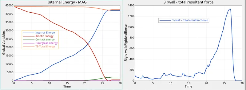
• The forces being plotted in the Rigid Wall Forces plot are the Usual Forces applied to the crash tube by the Rigid Wall. So as the contact energy increases, the Rigid Wall forces will also increase, and we can see that the Rigid Wall Forces also decrease at the point where the Contact energy flat and finally when the specimen loses contact with the Rigid Wall, the Rigid Wall Forces become Zero.

CASE 3: Create the type 11 contact and run.

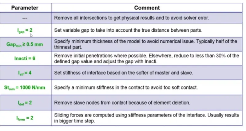
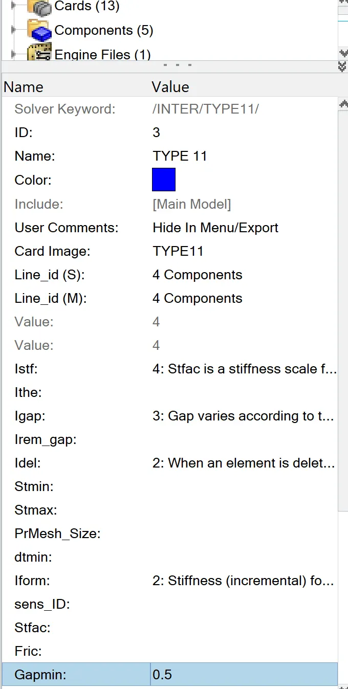
• In this case, we need to input type 11 interface to the case 2 solver deck file. After importing it in Hypermesh, Right-clicking the section, we can select Create >> Contact. After that, we can define this newly created contact and assign it the following values as shown below
• For both Line_id (S & M) attributes, all the components of the model will be selected. The other values are recommended settings for Type 11.
• Then, as usual, the file can be processed using the radioss solver. The remaining steps are followed as given.

• Now, run the analysis and open it in hyperview.

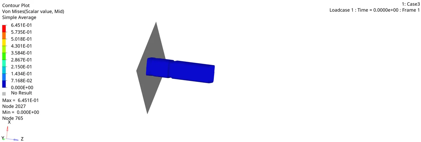
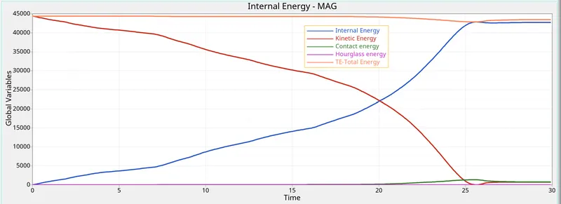
• The internal energy, which is representative of the energy absorbed, increases with time, as the tube contacts the rigid wall. We can observe a small peak and a drop off at around 26 seconds, which is the time when the tube is completely crushed and no more energy can be absorbed by the system.
• The hourglass energy is zero since the QEPH 24 element formulation has integrated hourglass control.

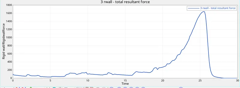
• Here, the deformation characteristics are like what was observed in previous cases. There is no discernible difference between the energy and rigid wall plots of this case and previous cases. Therefore, we can conclude that there was no edge-to-edge penetration in this model.

Case 4: Remove both notches and remove boundary condition on rigid body node then run.

• Import the 0000.rad file. Then remove the notch in the model using Align option. select reference nodes as 1st node and 2nd node. after that select the nodes that need to be aligned. now select align

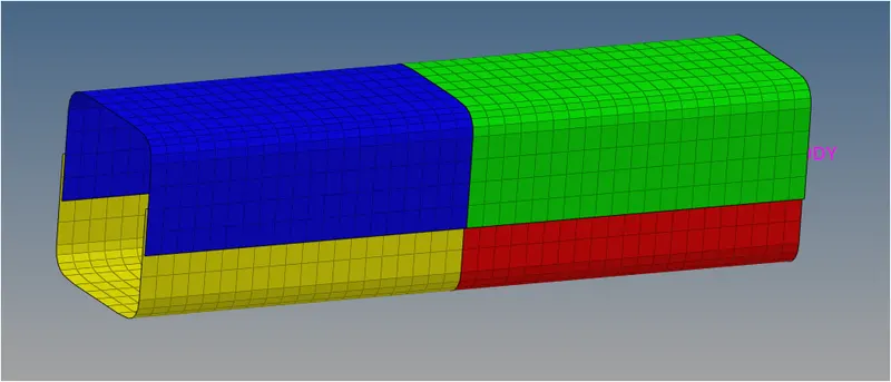
• There is no notch present in the model, the buckling started at the contact takes place in rigid wall and tube. In previous cases, buckling started at notch areas.
• Here we can switch to hypergraph 2D panel for plotting graph via client selector. In this panel, we need to load T01 file in file directory. Now select variable as Internal Energy, Kinetic Energy, total energy, contact energy, hourglass energy and select parameter as MAG and apply for plotting the graph.

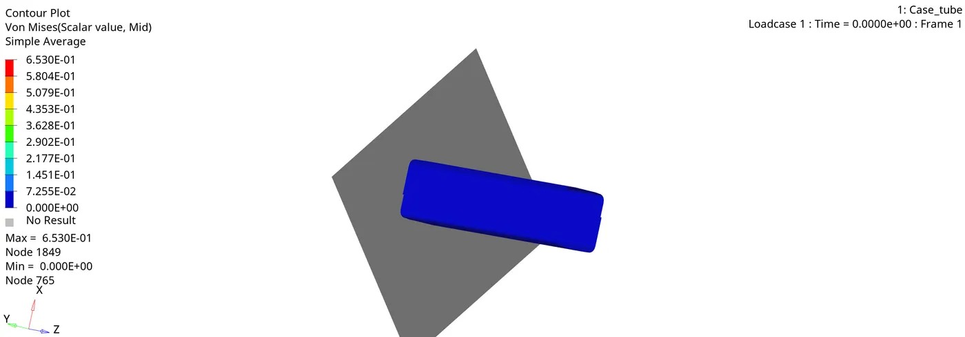
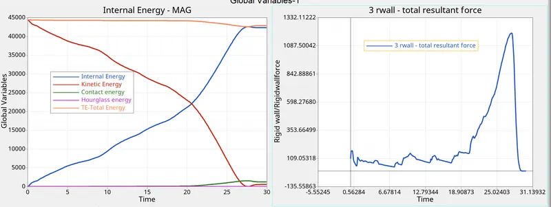
• Internal energy keeps increasing at some point due to the buckling of the tube. the more energy absorbed by the tube when deformation takes place. that's why the internal increases after some point.
• Kinetic energy decreases from maximum due to internal energy increases.
• Compared to previous cases, Contact energy slightly decreased after some point due to the absence of notches.
• Total energy also slightly decreased after some point due to contact energy. Hourglass energy is constant due to the presence of recommended properties.
• Next is to plot rigid wall resultant force graph for case 4 simulation, so select variable as rigid wall and parameter as resultant force and apply to plot the graph.
• In this case, the RWALL force graph peaks after some point due to a large amount of force is transferred to the rigid wall during the collision of the crush tube. After the deformation was completed, the graph decreased suddenly. and got a constant value after the deformation. The total resultant force peaks at 1350N.

CASE 5: Create a new notch in the middle ,select the whole section and run.

For this case, we shall be using the starter file of case 4. So, there are no notches or boundary conditions. But the case requires us to create a notch through the middle section of the crush tube. For this, I have used the translate tool in Hypermesh. Go to tools > translate.We can either select elements or nodes to translate. After assigning the direction of translation (using an axis or a vector), we then need to assign a magnitude. Depending on the global axis, we then must either click 'translate+' or 'translate-'. This creates the depression.

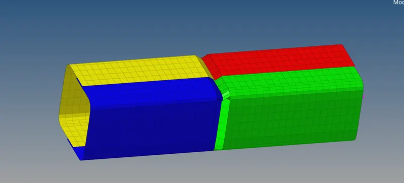
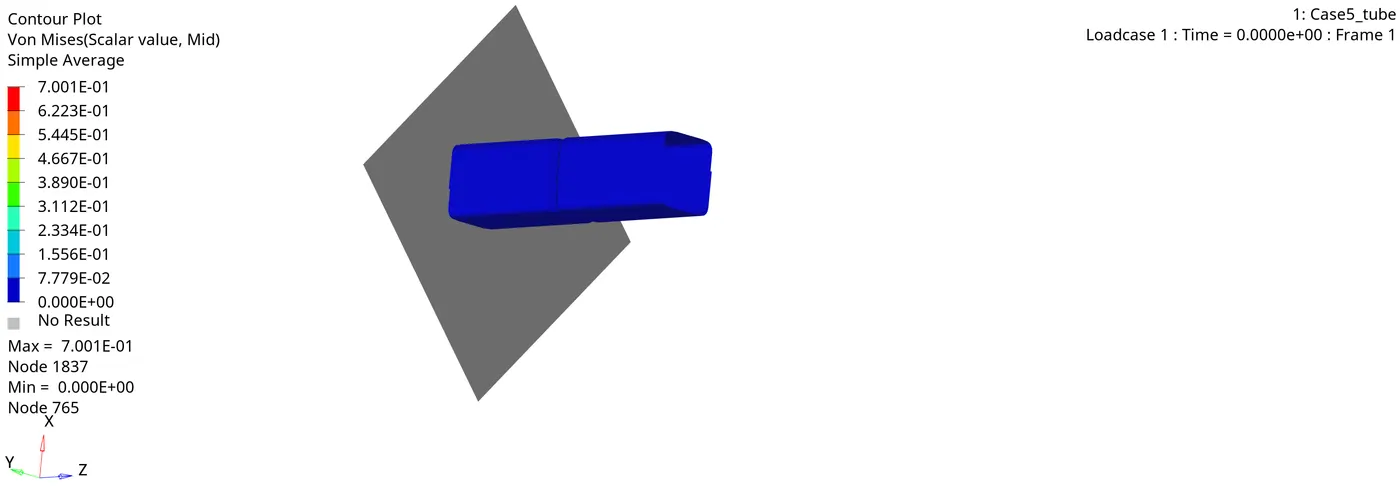
• Just as in the first 3 cases, the notch is the region where the tube undergoes deformation first. Then the region closer to the rigid wall is deformed next, which would be the lower half of the tube. Around the 8-12ms mark, when the lower half is mostly deformed, the upper half undergoes proper, visible deformation very rapidly until the entire tube is crushed completely.

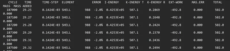
• Energy error is still within the -15% and present with 2.0%. Mass error is non-existent.

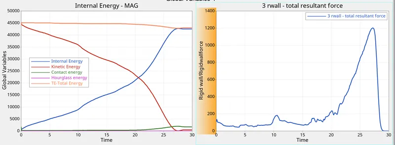
There is no immediate difference between case 4 and case 5 in these plot patterns other than the blip at around the 9 ms mark for the rigid wall plot. This happens specifically due to the complete buckling of the lower half of the crush tube. There is a small period where the tube transfers its capacity to absorb energy to the upper half and this is characterized by the slight increase and then decrease in rigid wall forces in that period.

As seen previously, the internal energy increases as kinetic energy decreases, and the increase in contact energy is more noticeable at an earlier point in time as compared to previous cases, this is probably due to the depth of the notches facilitating the buckling process.

CASE 6: Create a new notch with nodes only from opposing 2 faces and run.

For this case, we can make use of case 5's starter file and follow the same process of creating notches but instead of creating one all around the tube, we simply create two separate notches on opposing faces of the crush tube, using the same translate tool.

Now there are two sets of notches on the tube:

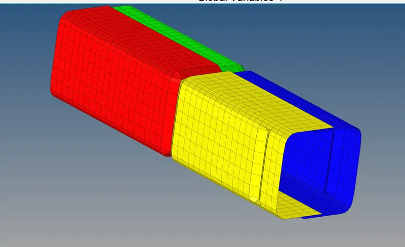
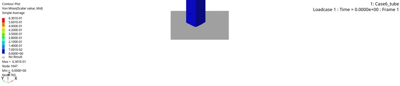
We can then carry out the analysis using radioss as outlined in the main procedure. The simulation is as follows:

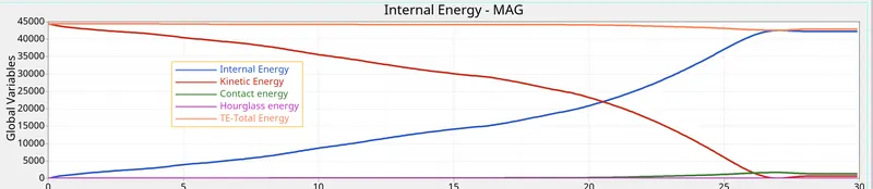
• Like in previous cases, the internal energy increases due to the deformation occur. kinetic energy decreases from high value due to increase in internal energy. The contact energy also noticeably increases due to the depth of the notch. Total energy increases due to contact energy increases after some point. Hourglass energy is constant due to the presence of recommended properties.
• Next is to plot rigid wall resultant force graph for case 6 simulation, so select variable as rigid wall and parameter as resultant force and apply to plot the graph.

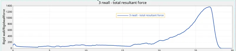
• Again, the plotted RWALL graph is similar like previous case. In this case, the peak value is slightly decreased due to the presence of notch only in opposing faces. After buckling process, the peak value drops to lesser and got constant after the tube crushed completely.

conclusions:

Notches are the regions where deformations happen first under duress, due to them being regions of stress concentration. But it does help to control and predict the location of deformations. This in turn plays a role in how the absorbed energy spreads throughout the tube. A notched tube results in higher contact forces but a smoother transmission of load.

In this assignment, different types of contacts were used to analyze the simulations of the crash tube. Under a constant load, the behaviour was observed by varying the geometry through the removal and creation of notches.

From all the cases we can say that criteria "Inacti" is required to be defined as it removes any initial intersections in the model if they exist. It helps to obtain a more accurate result and also reduces the no. of cycles & time taken to solve. The type 11 contact is given between 2 edges and requires lesser parameters to be defined and also takes comparatively lesser time to be solved than a type 7 contact.