Assignment 4-RADIOSS Material Laws Challenge

AIM:

    To run crash analysis on the given model by applying different materials laws available in Radioss and post-process the results

OBJECTIVE:

    To carry out simulations with the given starter files and compare the results. There are 7 cases listed (according to given parameters) to be analyzed and compared  and they are to be compared based on the Von Mises Stress and Energy deformations. The files that are to be imported for the analysis are FAILURE_JOHNSON_0000.rad file and LAW27_0000.rad file.

The cases to be analyzed and compared are as follows:

1. LAW 2 (file - FAILURE_JOHNSON_0000.rad) Base simulation.
2. LAW 2 (file - FAILURE_JOHNSON_0000.rad) with Ifail_sh = 1, Dadv = 1, and Ixfem = 1.
3. LAW 2 (file - Starter file from Case 2) with fail/JOHNSON card deleted.
4. LAW 2 (file - Starter file from Case 3) with EPS_p_max value deleted.
5. LAW 1 (file - FAILURE_JOHNSON_0000.rad) with fail/JOHNSON card deleted and values for density, E, nu to be assigned.
6. LAW 27 (file - LAW27_0000.rad) with recommended shell properties.
7. LAW 36 (file - LAW27_0000.rad) with recommended shell properties and given reference curve.

THEORETICAL CONTENT:

• The accuracy of the simulation depends on the material chosen.
• Choosing the right material and providing the reliable material data in performing a simulation is very important.
• RADIOSS has multiple material properties and wide variety of material library like concrete, foam, rubber, composites etc.,
• Some of the commercially used material laws are:

1. Law 1: Elastic (Isotropic Elasticity)
2. Law 2: Johnson-Cook (Isotropic Elasto-plastic)
3. Law 27: Elasto-plastic brittle
4. Law 36: Elasto-plastic tabulated
5. Law 42: Ogden (Visco Hyperelastic)
6. Law 70: Foam

LAW 1: Isotropic Elasticity

• Isotropic means that a material will have the same material properties in all 3 directions.
• The RADIOSS elasticity law follows the hooke’s law of elasticity (i.e)., a linear relationship between the stress and strain.
• It is available for truss, beam, shell and solid elements. As mentioned earlier, it is exclusively suitable for elastic materials.
• The material stiffness is determined by Young’s modules of elasticity (E) and Poisson’s ratio (nu).
• The sheer modulus G is calculated by G = E / 2*(1+V)

Description	Model Name	Keyword/MAT	Model Law
Linear Elastic	Elastic [Hooke's]	/ELAST	1
Hyper Elastic	Tabulated Hyper Elastic	NA	69
Hyper Elastic	Ogden	NA	82

Limitations:

• Elastic materials cannot be used for large deformation cases such as blow molding etc.
• In the case of large deformation, Law 2 - Johnson-Cook material with high yield can be used.

LAW 2: Isotropic Elasto-Plastic

• RADIOSS provides various types of elasto-plastic material laws. It has all the material models based on Von mises hardening without damage, Von mises hardening with ductile damage and Von mises with visco-plastic flow.
• Here the material laws used are Johnson-Cook/JOHNS and tabulated piece-wise linear/PLAS_TAB.

Johnson-Cook Material (PLAS_JOHNS):

• This law represents an isotropic elasto-plastic material using the Johnson-Cook Material model.
• The model expresses material stress as a function of strain, strain rate and temperature.
• In the material card, we have an option called EPS_max which is nothing but plastic strain at failure. Failure of the element happens when 1 integration point reaches EPS_max.
• Now if failure is only based on EPS_max, there can be instances where the EPS_max gives out unrealistic results. To avoid this we have the option called /FAILS/JOHN.
• /FAILS/JOHN card provides the user with more control over the failure of the Johnson-Cook strain.

LAW36: PLAS_TAB Elasto-plastic piecewise linear material

• The LAW36 material law helps in modelling isotropic elasto-plastic material using user defined functions for the work hardening portion of the stress-strain curve for different strain rates.
• The curve defined is nothing but the stress-strain curve after the yield point. The yield point is set to 0 and this material law is available for both brick and shell elements.
• If the work hardening portion is defined by the user, then its elastic portion is taken from the input Young's modulus (E) and Poisson's ratio (nu).
• Any number of stress-strain curves can be defined. The important point is that the strain rate curves must not intersect with each other.
• The plastic strain curve should start with 0. The user also has an option to provide yield stress input value with respect to pressure using fct_Idp.

There are 4 damage and rupture parameters :

• εpmax">εpmax is the maximum plastic strain for element deletion for any loading (tensile , shear or compression).
• εt is the beginning of tensile damage. From this point the stress value defined in the curve is reduced by the factor
• Where ε1 is the largest principal strain σ=σ(εm-ε1/εm-εt)">σ=σ(εm−ε1/εm−εt)σ=σ(εm-ε1/εm-εt).
• εm is the end of the tensile damage. The stress value is null, but the element is not deleted.
• εf is the tensile failure strain value for element deletion.

LAW 27: Elasto-Plastic Material with Brittle Failure

• This law combines an isotropic elasto-plastic Johnson-Cook material model with an orthotropic brittle failure model.
• Material damage is accounted for prior to failure. Failure and damage occur only in tension. This law is applicable only for shells.
• Yield surface definition same as Johnson-Cook (Law2).
• Useful for modeling brittle failure of glass.
• Damage and rupture defined with 4 parameters for each principal direction:
  et">et = Strain at the beginning of tensile failure.
  em">em = Maximum tensile strain at which the stress in the element is set to a value dependent on dmax1.
  dmax">dmax = Maximum damage factor ef = Maximum tensile strain for element deletion.

Viscous Material:

The viscous materials are classified into two types called Hyper Elastic /MAT/OGDEN or /MAT/LAW42 : Ogden, Mooney-Rivlin & Tabulated Foam /MAT/FOAM_TAB or /MAT/LAW70.

LAW 42: Hyper Elastic /MAT/OGDEN or /MAT/LAW42 - Ogden, Mooney-Rivlin

• They are Visco Hyperelastic behavior (non-linear elastic). 
• This law is generally used to model incompressible rubbers, polymers, foams, and elastomers.
• This material can be used with shell and solid elements.
• Generally used to model polymers and elastomers.

LAW 70: Tabulated Foam /MAT/FOAM_TAB or /MAT/LAW70

• Visco-elastic behavior
• Stress – strain relationship defined by functions according to strain rate
• Unloading behavior defined by:

1. Curves 
2. Hysteresis Parameters

PROCEDURE:

Importing the file:

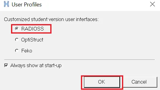
• Open Hyper mesh, Go to ⟹ Import ⟹ Solver deck option ⟹ Browse File ⟹ Import. The “FAILURE_JOHNSON_0000.rad” file is selected and “imported” as shown below.

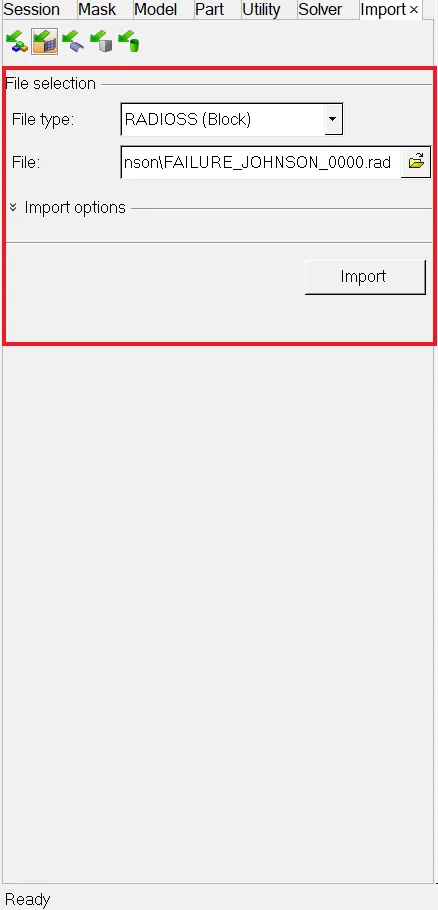
• Here the import browser will appear as shown and select the appropriate starter file to import into GUI.
• Switch the File Type to Radioss Block and import the model into GUI.
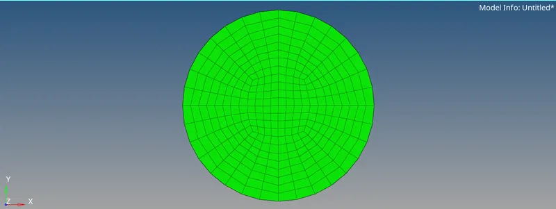
• Here the model is in wireframe mode,Switch to the shaded mode as shown below.
• To switch to shaded mode, Go to Visualization Tab ⟹ Shaded Elements and Mesh Lines.

Running the simulation:

Case 1 - LAW 2 (file - FAILURE_JOHNSON_0000.rad) Base simulation :

• Now after importing the model into the GUI,Go to the solver browser and select the begin card to inorder to check the unit system and check the material card by selecting it in model browser inorder to check whether the appropriate properties have been assigned or not,The material property card is shown in below.

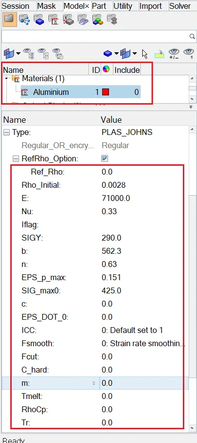
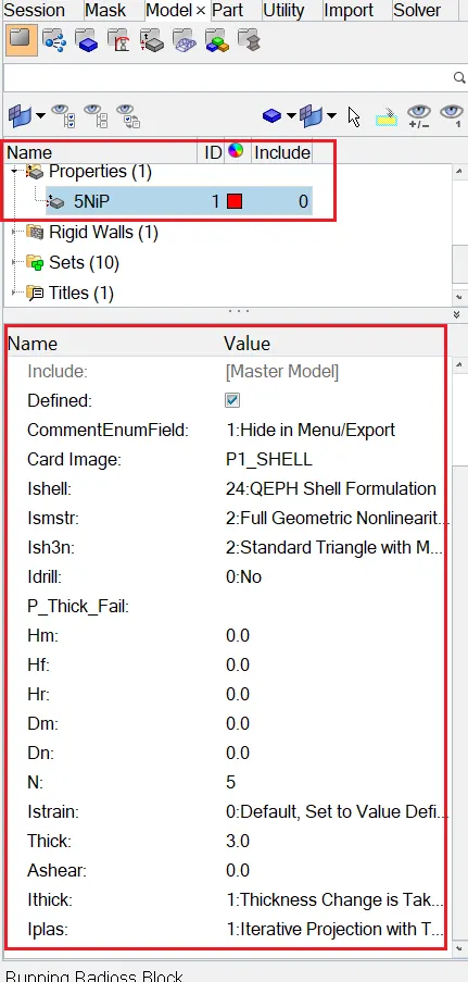
• Now go and check the property card.In the property the parameters have been assigned to the material given,Which is shown in below.

• Now run the simulation,To run simulation,Go to Analysis Panel as shown in figure 28.
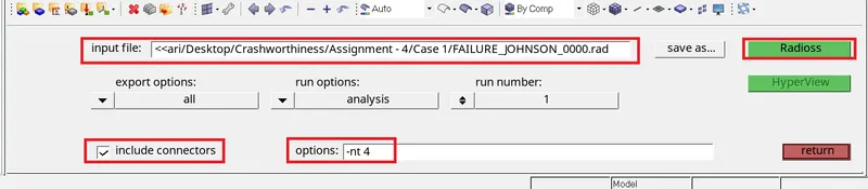
• Go to Analysis Panel ⟹ Radioss ⟹ Select the Input File ⟹ Save it in Different Folder ⟹ Run.
• Check the Include Connectors,If there are any connectors in the model,The connectors will also be taken into account.
• Type -NT 4 in options tab,This will make the simulation faster.
• Where NT indicates No of threads,4 indicates assigning the task to 4 cores in the system.
• Here save the input file in a different folder after renaming it and run the solver by hitting on radioss.

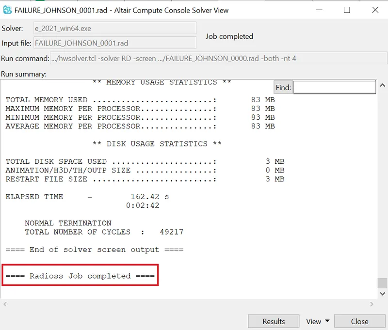
• After completing the simulation,the radioss will pop up a solver window stating Radioss Job Completed which indicates the simulation has been completed, which is shown below.

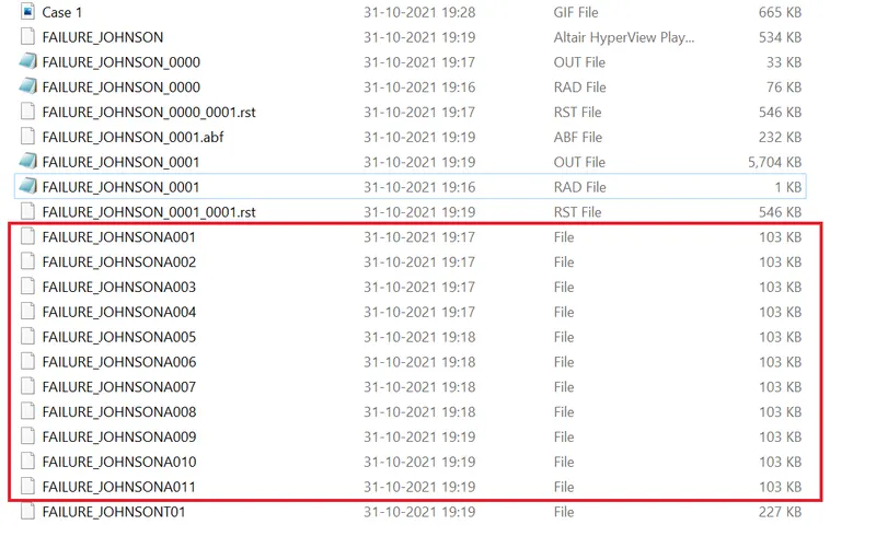
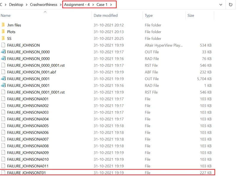
• After running the simulation,The animation files will be generated where we specified a location to store the files which is shown in below.

• Now go and open the 00001.out file with notepad. The obtained values for Energy Error,Mass Error,Internal Energy Error,Kinetic Energy Error and Contact Energy Error has been shown below.

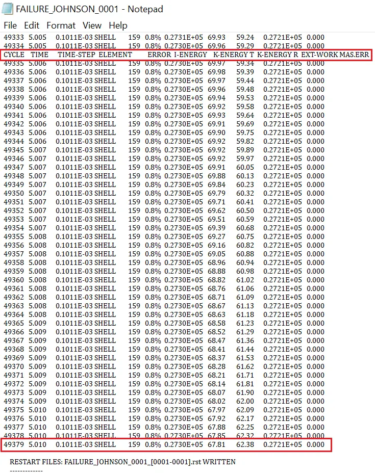
• The values obtained for this cycle are

• Energy Error-0.8%
• Internal Energy-0.2730E+05
• Kinetic Energy-67.81
• External Work-0.2721E+05
• Elapsed Time-95.36s
• Mass Error-0
• Total No of Cycles-49380

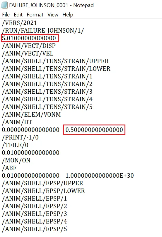
• Next the 00001.rad file is opened to see the Tstop and Tfrequency value which is shown in below.

Postprocessing

• Review the Simulation using -HyperView.
• Plot the graphs using -Hypergraph 2D.

Review the Simulation using HyperView:

• Hyperview allows for loading and viewing result files obtained from several sources.
• Based on the solver type of the files and the results you would like to visualize and analyze,there are differnt ways to load the input deck and their corresponding results into hyperview.
• First to begin the postprocessing in the Hypermesh,Split the Screen as shown below. Import the animation file .h3d into the hyperview.

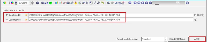
• To access the load model panel, select Load Model Button from the HyperView Panel and open .h3d file. 

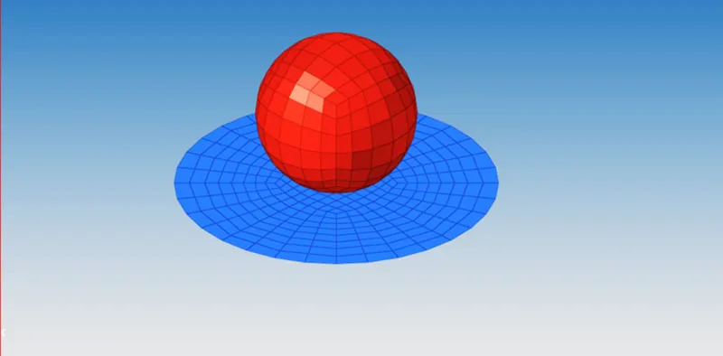
• After loading the model into hyperview, it will be represented as shown below.

• After importing the .h3d file into the GUI,Enable the contour.
• The contour tool create contour plots of a model graphically visualize the analysis results.
• To enable contour, Go to Results ToolBar ⟹ Contour .
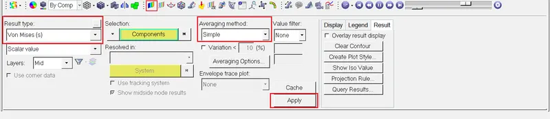
• Now switch to the Von Misses Stress in result type and select the component,select the averaging method as simple and then click apply as shown below.

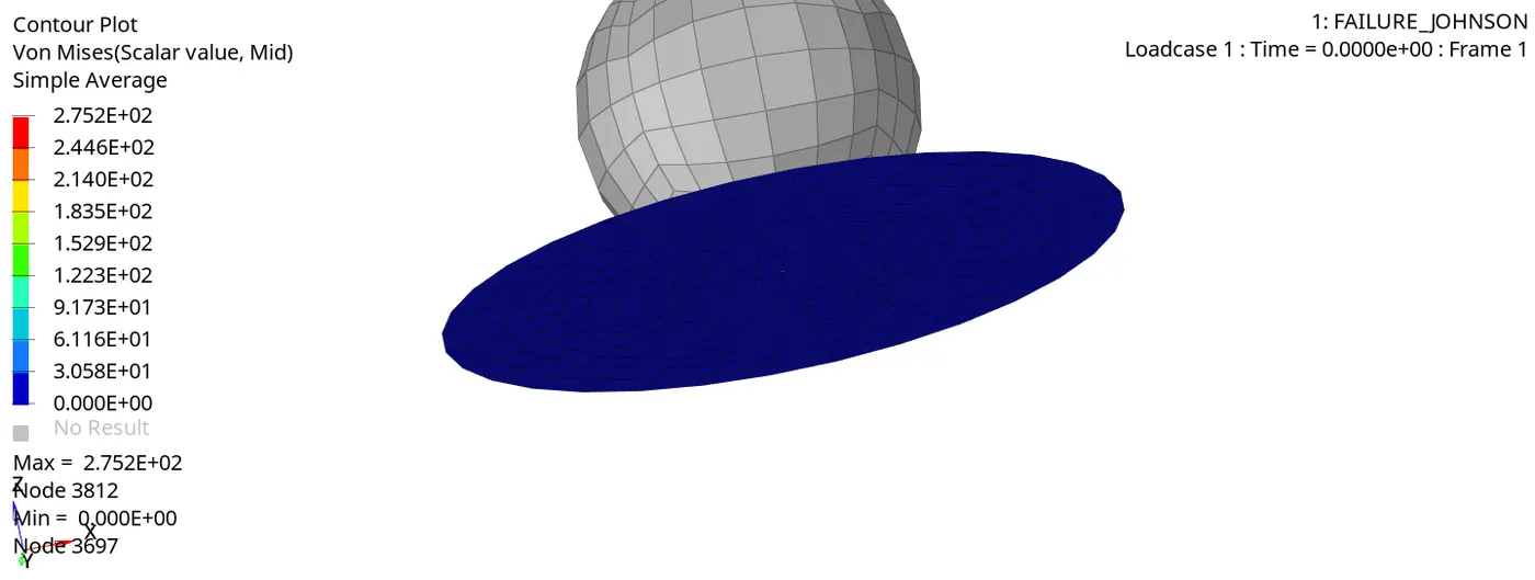
• After applying ,Run the Simulation,The Simulation animation is shown below.

Plot the graphs using Hypergraph 2D:

• Now plot the graphs using Hypergraph 2D,We are plotting the graphs to see what is happening in the rail component.
• Hypergraph 2D is a powerful data analysis and plotting tool with interfaces to many popular file formats.
• It is sophisicated math engine capable of processing even the most complex mathematical expressions.
• Hypergraph 2D combines these features with high quality presentation output and customization capabilities to create a complete data analysis system for any organization.

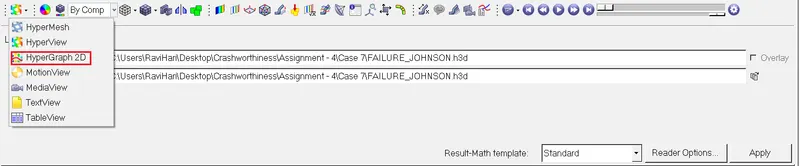
• Here switch to the Hypergraph 2D to plot the graphs.
• To switch, Go to Client Selector ⟹ Choose the Hypergraph 2D as shown above.
• The first graph is plotted for the Rigid Wall Forces.
• To plot the graph,Go to Hypergraph 2D ⟹ Data File ⟹ Element_Formulation-Shell-3_assignmentT01 ⟹ Apply.

• Here the graph has been plotted for the Rigid Wall Forces as shown below.
• There are various parameters in Rigid Wall like Normal Force,Tangent Force,FX-X Total Force,FY-Y Total Force,FZ-Z Total Force,Total Resultant Force. Here we go by selecting the Total Resultant Force option as we do not know the exact axis of the component placed.

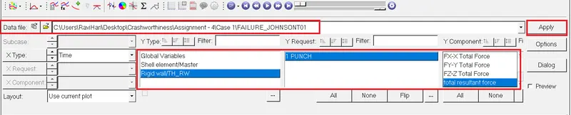
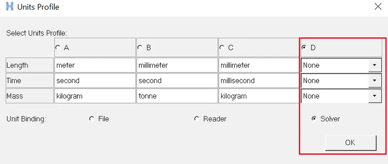
• While plotting the graph,Units profile window will pop up,There select solver units and then plot the graph,Because the graphs will be plotted according to the solver units.
• Now plot the graph for the rigid wall forces which is shown below.

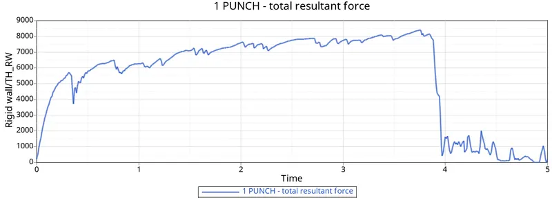
• Here,Intially there is no contact between the plate and rigid wall.So the curve is in origin.
• When the rigid ball hits on the rupture plate,the curve starts increasing and suddenly the curve starts decreasing.
• Because after reaching the ultimate stress, the elements gets deleted and there will be no contact after the elements get deleted which is shown above - Case 1: Simulation Animation and thus the curve goes down and decreasing.
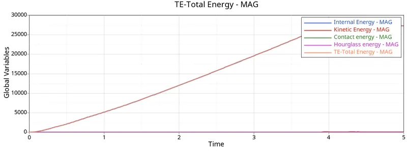
• Now plot the graphs for all the energies which is as shown below.

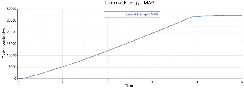
Internal Energy:

• Here the internal starts from origin why because there is no contact between rigid ball and rupture plate.
• Then the internal energy goes on increasing because the deformation or displacement is happening only and thus when the displacement increases the internal energy increases.

Kinetic Energy:

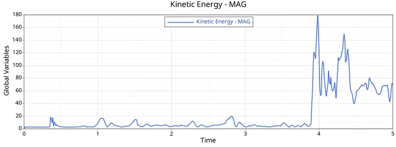
• Here the kinetic energy is in origin,Why because there is no initial velocity,there is a imposed velocity.
• The impose velocity is for rigid ball,Why because we are imposing the rigid ball to hit on the rupture plate,So that's the reason,why impose velocity is given.
• Here the initial velocity is zero, so the curve starts from origin.
• After its increasing because rigid ball is hitting rupture plate and again its slightly decreasing due to element breakage. After the elements are deleted, there will be no contact and so it is decreasing.

Total Energy:

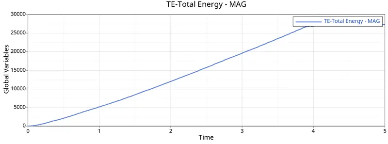
• Total Energy is sum of Kinetic Energy+Contact Energy+Hourglass Energy + Internal Energy.
• Total Energy is the combination of all energies.
• So its goes on increasing,Internal energy curve is similar to the total energy.

Contact Energy:

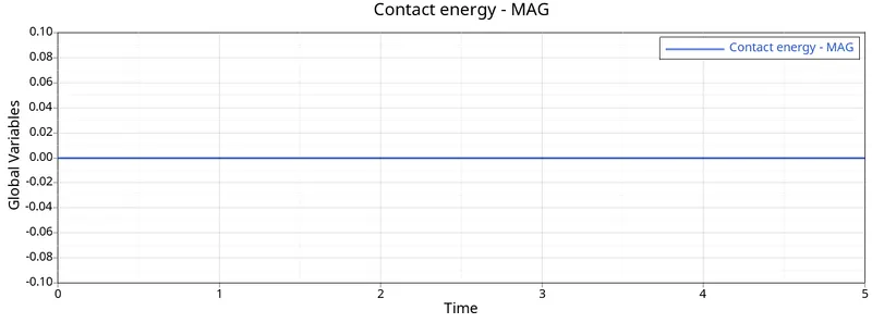
• As the rigid ball is rigid body and the rupture plate is deformable body so that the contact energy is constant.
• If deformable bodies get in contact,then only the contact energy increases.

Hourglass Energy:

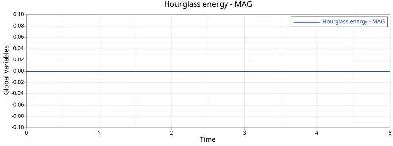
• Here the hourglass energy is constant,Because the recommended parameter Ishell=24 has been assigned to the property card,So the hourglass energy is constant.

Processed Models:

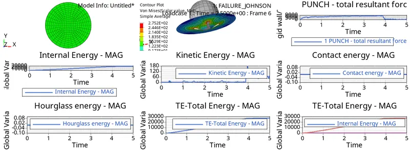
Case 2 - LAW 2 (file used - FAILURE_JOHNSON_0000.rad) with Ifail_sh = 1, Dadv = 1, and Ixfem = 1:

• Here the Jhonsons Failure card is edited,and the values have been given in the failure card as per the values given the question.
• But the law is same [LAW 2],Only the failure card is edited.
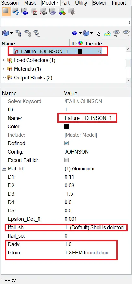
• The values which are to be changed are Ifail_sh=1,Dadv=1,Ixfem=1.
• Here ~Dadv = 1 - Initiate the crack when it reaches ultimate stress.
          ~Ifail_sh = 1 -Shell is deleted or cracked, if there is one layer in the failure zone.
          ~Ixfem = 1 - Crack the elements and delete the elements. (Ixfem is only applicable for shell elements).
• The values have been given as input in the failure card which is shown below

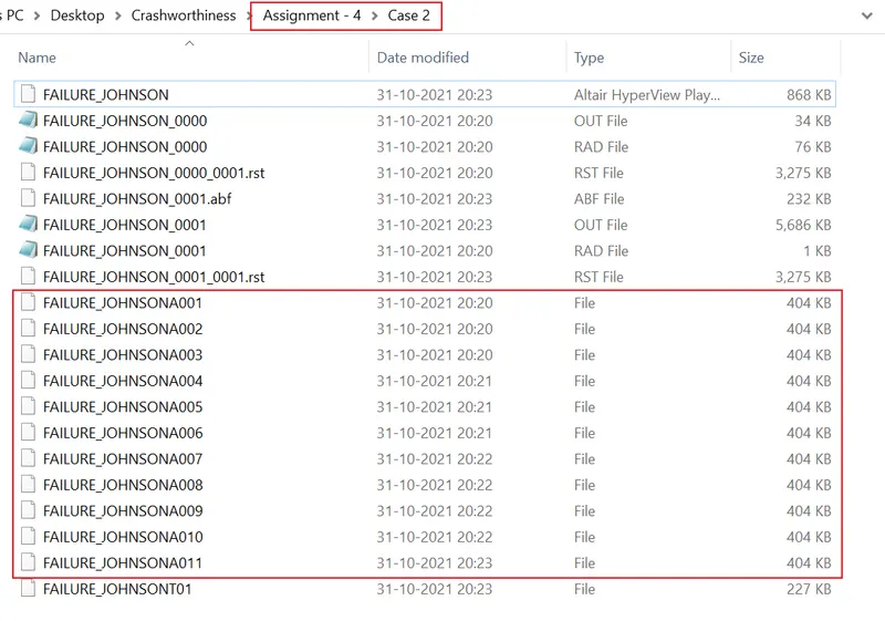
• Now run the simulation using radioss,After running the simulation,The animation and TH files will be obtained in a required location,which is shown below

• Now go and open the 00001.out file with notepad.
• The obtained values for Energy Error,Mass Error,Internal Energy Error,Kinetic Energy Error and Contact Energy Error has been shown below.

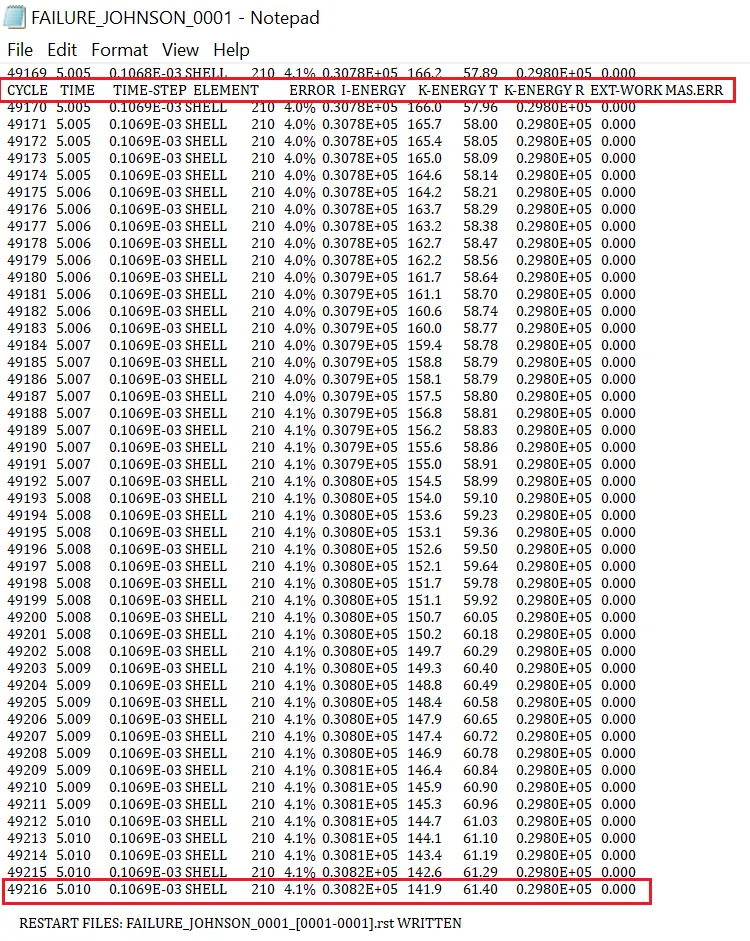
• The values obtained for this cycle are

• Energy Error-4.1%
• Internal Energy-0.3082E+05
• Kinetic Energy-141.9
• External Work-0.2980E+05
• Elapsed Time-134.34s
• Mass Error-0
• Total No of Cycles-49217

Review the Simulation using HyperView:

• After completion of running the simulation,Switch to the hyperview.
• Open the appropriate .h3d file to review the simulation.
• The .h3d file is loaded and it is shown below.

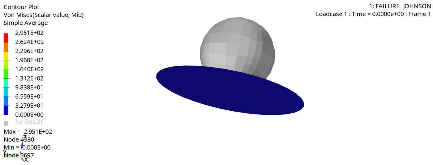
• Here the value given in material card for Eps_p_Max = 0.151 so that the elements should be deleted after reaching the Eps_Max = 0.151. 
• But here the maximum strain recorded is 0.147 and the elements gets deleted in this point itself and thus the solver won't record till the value of 0.151.
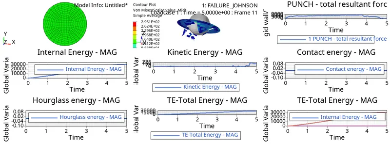
• The elements will be failing and getting deleted when the rigid ball goes on hitting the rupture plate.

Plot the graphs using Hypergraph 2D:

• Now switch to the Hypergraph 2D and plot the graphs.

Rigid Wall Forces:

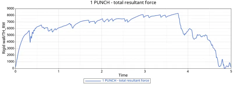
• Here the curve starts from origin,because there is no contact and it goes on increasing because the deformation happens (rigid ball comes into the contact with rupture plate).
• Again its suddenly decreasing,Cause the elements are cracked and deleted,there will be no contact between rigid ball and rupture plate,So its slightly decreasing.

Internal Energy:

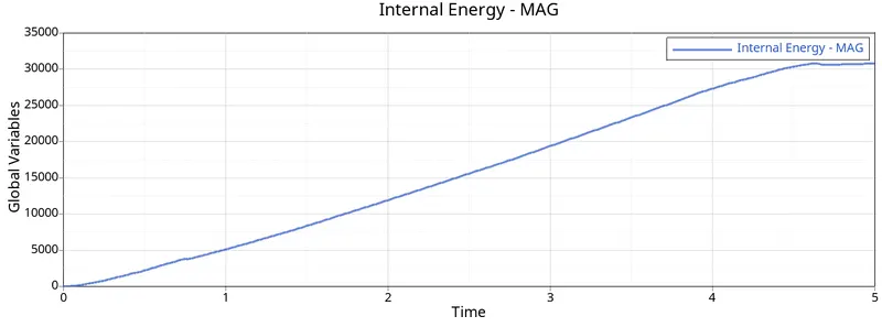
• Here the curve is starting from origin because there is no contact and its goes on increasing due to the breakage of elements.

Kinetic Energy:

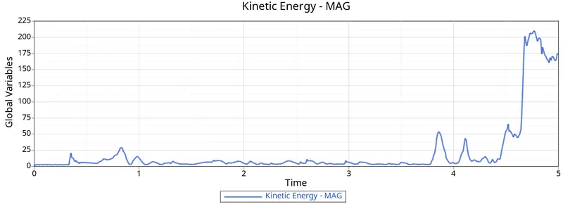
• Here the kinetic energy starts from origin and goes on increasing due to deformation of elements,Its increasing after 4ms because the deformation of elements are controlled by Jhonson-Cook material parameters. And its suddenly decreasing because the elements getting deleted after crack and there will no contact,so its slightly decreasing.

Total Energy:

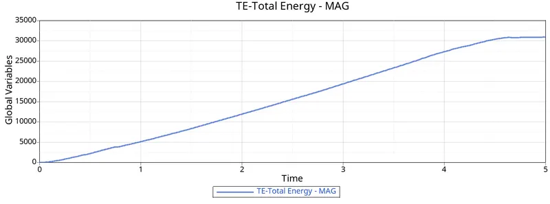
• Total Energy is sum of Kinetic Energy+Contact Energy+Hourglass Energy + Internal Energy.
• Total Energy is the combination of all energies.
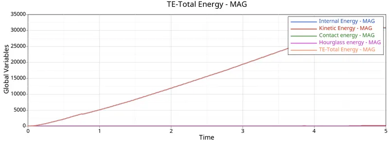
• So its goes on increasing, Internal energy curve is similar to the total energy.

Hourglass Energy:

• Here hourglass energy is constant due to recommended parameters have been assigned.Here Ishell=24 QEPH is used,Due to this there is no houglass effect.

Contact Energy:

• As the rigid ball is a rigid body and the rupture plate is a deformable body, the contact energy is constant.
• If deformable bodies get in contact, then alone the contact energy increases.

All Energies:

Processed Models:

 

Case 3 - LAW 2 (file used - Starter file from Case 2) with fail/JOHNSON card deleted:

• Here the failure card is deleted to see any changes happening in the results.

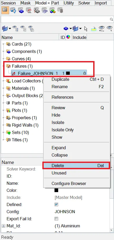
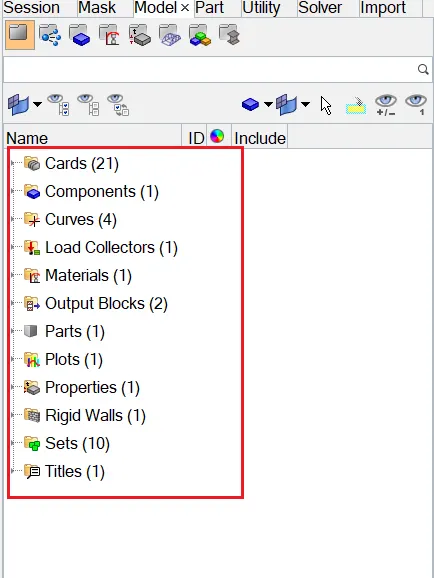
• We could observe that the failure card is deleted from the model browser.

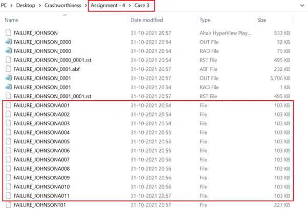
• Now run the simulation using radioss, the animation and TH files will be saved in the specified location which is shown below.

 

• Now go and open the 00001.out file with notepad.
• The obtained values for Energy Error,Mass Error,Internal Energy Error,Kinetic Energy Error and Contact Energy Error has been shown below.

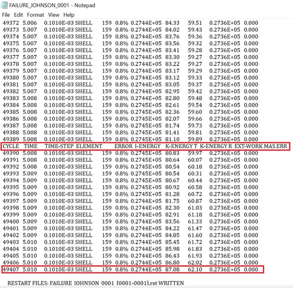
• The values obtained for this cycle are

• Energy Error-0.8%
• Internal Energy-0.2744E+05
• Kinetic Energy-87.08
• External Work-0.2736E+05
• Mass Error-0
• Elapsed Time- 96.79 s
• Total No of Cycles-49407

Review the Simulation using HyperView:

• After completion of running the simulation ⟹ switch to the hyperview.
• Open the appropriate .h3d file to review the simulation.
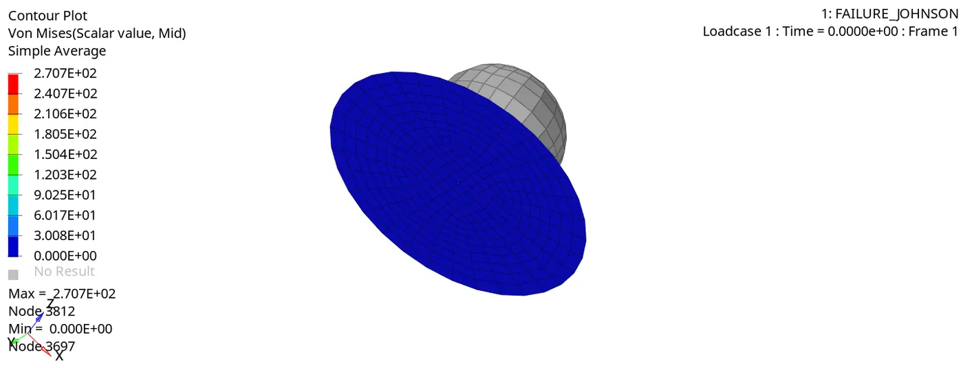
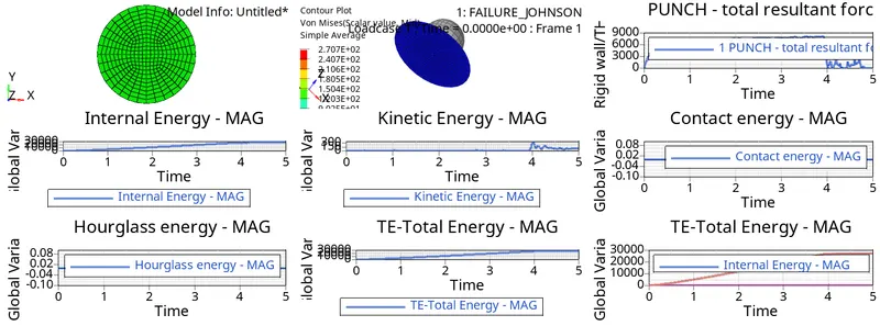
• The .h3d file is loaded and it is shown below. Here the shell elements are getting deleted when it reaches the maximum plastic strain Epsmax value which is shown below.

Plot the graphs using Hypergraph 2D:

Rigid Wall Forces:

• Now switch to the Hypergraph 2D and plot the graphs.
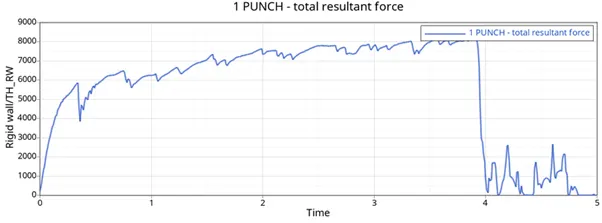
• The rigid wall forces graph is plotted which is shown below. Here the graph plotted for the Case-3 rigid wall forces is very similar to Case-1 rigid wall forces.

Internal Energy:

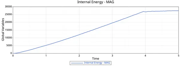
• The internal energy graph is plotted which is shown below.
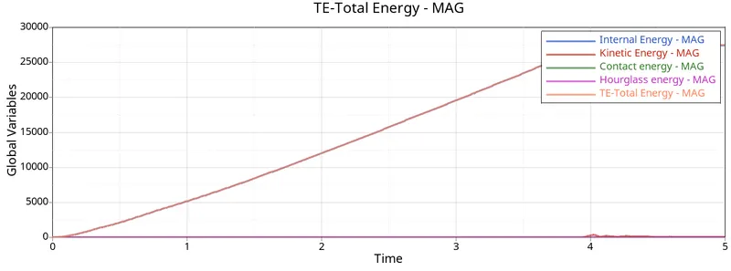
• Here the internal energy is almost similar to the previous cases 1 & 2.

Kinetic Energy:

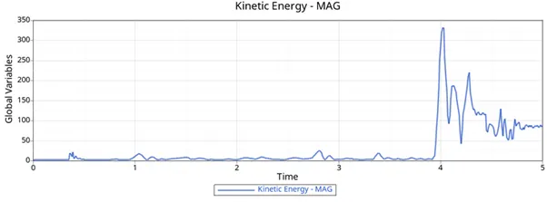
• The kinetic energy obtained here is somewhat less when compared to the previous case and the resultant kinetic energy graph is as shown below.

Total Energy:

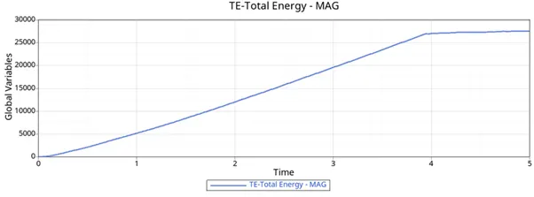
• The total energy increases with increase in internal energy and kinetic energy as the total energy is combination of all energies.
• The obtained total energy graph is shown above. 

Hourglass and Contact Energy:

 

• Here hourglass energy is constant due to recommended parameters have been assigned. Here Ishell = 24 QEPH is used. Due to this there is no houglass effect.
• As the rigid ball is a rigid body and the rupture plate is a deformable body, the contact energy is constant here. Only if deformable bodies get in contact the contact energy will increase.
• The obtained hourglass and contact energy graph is shown above.

All Energies:

Processed Models:

 

Case 4 - LAW 2 (file - Starter file from Case 3) with EPS_p_max value deleted:

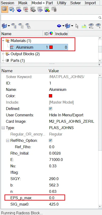
• Here delete the value of EPS_P_Max value and run the model with the name LAW2 but the same material card.
• The value of plastic strain is removed which is shown in below.

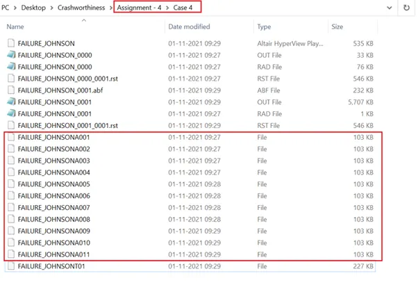
• Now run the simulation using radioss, the animation and TH files will be saved in the specified location which is shown below.

• Now go and open the 00001.out file with notepad.
• The obtained values for Energy Error,Mass Error,Internal Energy Error,Kinetic Energy Error and Contact Energy Error has been shown below.

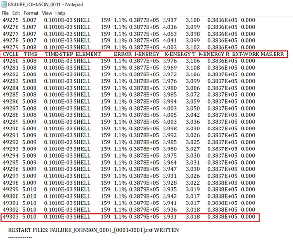
• The values obtained for this cycle are

• Energy Error-1.1%
• Internal Energy-0.3879E+05
• Kinetic Energy-3.931
• External Work-0.3838E+05
• Mass Error-0
• Elapsed Time- 131.47s
• Total No of Cycles-49303

Review the Simulation using HyperView:

• After completion of running the simulation then switch to the hyperview.
• Open the appropriate .h3d file to review the simulation.
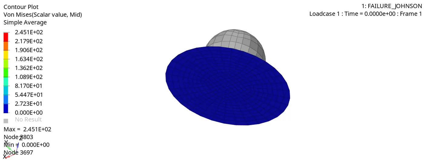
• The .h3d file is loaded and it is shown below.
• Here EPS_p_max = 0, so that the shell elements will not be deleted which is as shown below.

Plot the graphs using Hypergraph 2D:

• Now switch to the Hypergraph 2D and plot the graphs.
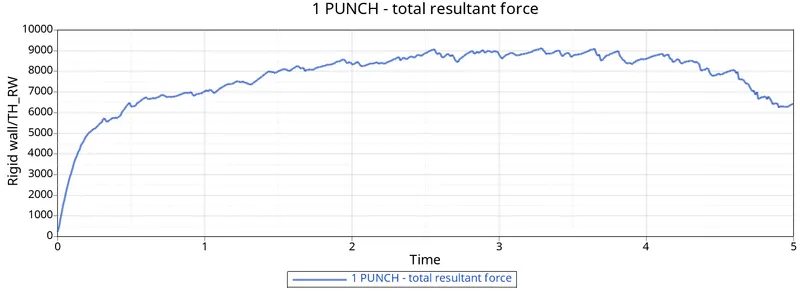
• The rigid wall forces graph is plotted which is shown below.

Rigid Wall Forces:

• Here the rigid wall forces starts from origin cause there will be no contact in the beginning and it goes on increasing cause deformation is happening to the plate.
• And the curve slightly decreases because of the elements breakage.

 

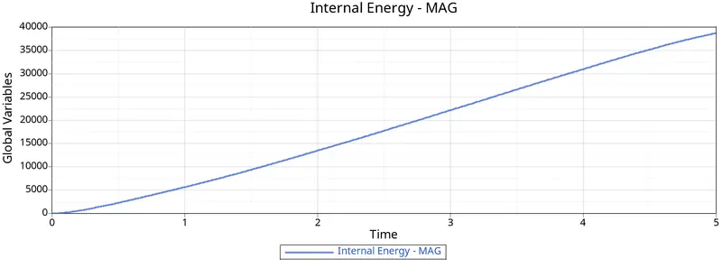
Internal Energy:

• The internal energy graph is plotted which is shown below and the plotted graph here for internal energy is almost similar to the previous case.

Kinetic Energy:

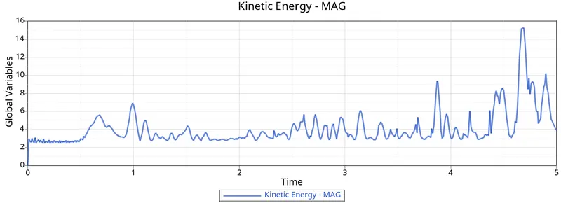
• The kinetic energy is plotted and the kinetic energy graph is also similar to the previous case.
• Kinetic Energy produced here is slightly less as the deformation of elements is happening at a slow rate.

Total Energy:

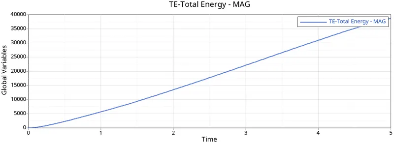
• The total energy is almost similar to the internal energy.
• The total energy graph is plotted which is shown below.

Hourglass and Contact Energy:

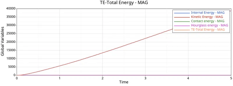
• Here hourglass energy is constant due to recommended parameters have been assigned.Here Ishell = 24 QEPH is used. Due to this there is no houglass effect.
• Because the rigid ball is rigid body and the rupture plate is deformable body and thus the contact energy is constant.
• If deformable bodies get in contact,then only the contact energy increases.
• The obtained hourglass and contact energy graph is shown above.

All Energies:

Processed Models:

 

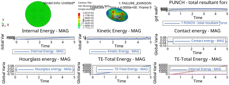
Case 5 - LAW 1 (file - FAILURE_JOHNSON_0000.rad) with fail/JOHNSON card deleted and values for Density, E, nu to be assigned:

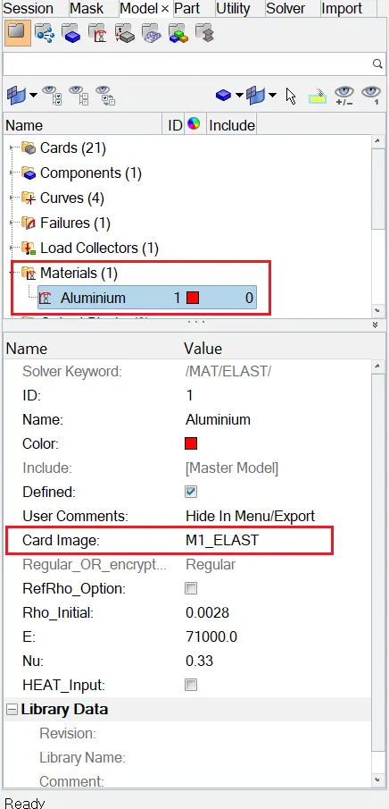
• Here change the material card to LAW1, here it will be elastic behaviour.
• Don't change any material properties, use default material properties like density, Young's modulus and Poissons ratio.

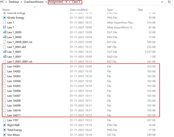
• Now run the simulation using radioss, the animation and TH files will be obtained in a required location which is shown below.

• Now go and open the 00001.out file with notepad.
• The obtained values for Energy Error,Mass Error,Internal Energy Error,Kinetic Energy Error and Contact Energy Error has been shown below.

 

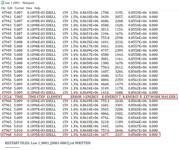
• The values obtained for this cycle are

• Energy Error- -7.4%
• Internal Energy-0.7195E+06
• Kinetic Energy-425.7
• External Work-0.7780E+06
• Mass Error-0
• Elapsed Time- 117.85s
• Total No of Cycles-47900

Review the Simulation using HyperView:

• After completion of running the simulation,Switch to the hyperview.
• Open the appropriate .h3d file to review the simulation.
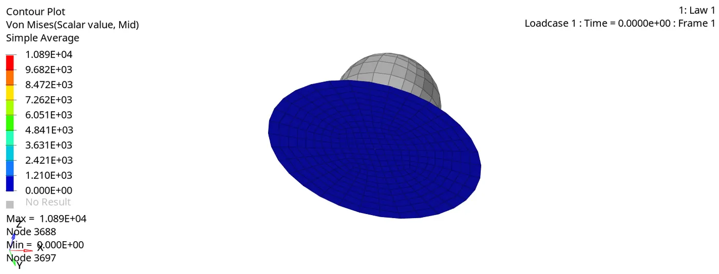
• The .h3d file is loaded and it is shown in below and here EPS_p_max = 0, So the shell elements will not be deleted which is shown below.
• The elements will not even split during the collison as the LAW1 material card is assigned to the rupture plate.
• So there will be an elastic behaviour (ability to regain its original size and shape).

Plot the graphs using Hypergraph 2D:

• Now switch to the Hypergraph 2D and plot the graphs.
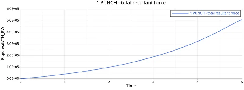
• The rigid wall forces graph is plotted which is shown below.

Rigid Wall Forces:

• Here the rigid wall forces starts from origin cause there will be no contact in the beginning and it goes on increasing cause deformation is happening to the plate.
• And the elements not getting deleted here and thus its goes on increasing till to end.

Internal Energy:

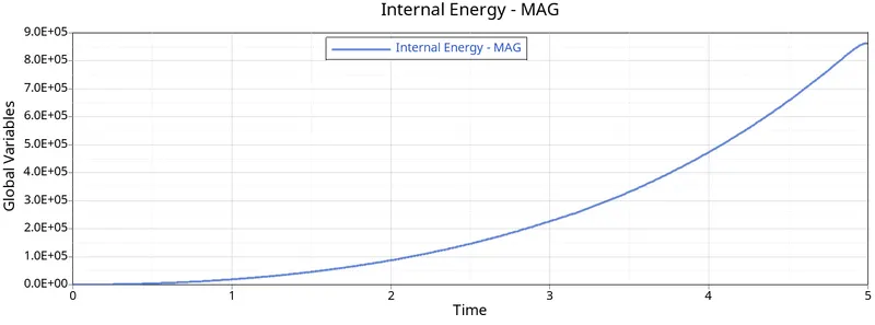
• Here the internal energy starts from origin because in the beginning ,the rigid ball is not in contact to the plate.
• Its increasing when the rigid ball hits the rupture plate, its goes on increasing.
• The graph obtained for internal energy is shown below.

Kinetic Energy:

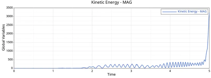
• Here kinetic energy is in initial condition,so its starts from origin.
• It increases when the rigid ball hits the rupture plate.
• And its slighlty decreasing,because after hitting the rupture plate,the rigid ball goes back to its position and there will be no contact.

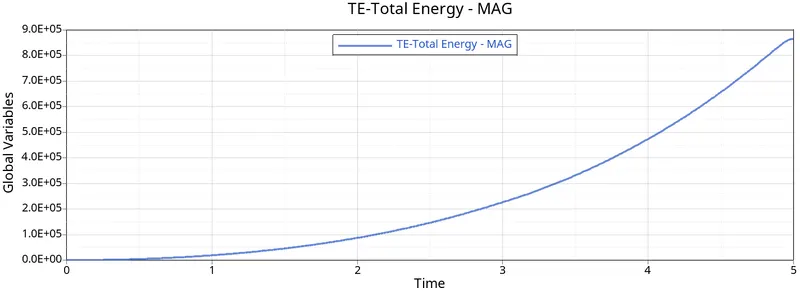
Total Energy:

• The total energy increases with the increase in kinetic energy and internal energy and thus the graph obtained for total energy is shown below.

 

Hourglass and Contact Energy:

• Here hourglass energy is constant due to recommended parameters have been assigned. Here Ishell = 24 QEPH is used and hence there is no houglass effect.
• Because the rigid ball is rigid body and the rupture plate is deformable body, So the contact energy is constant.
• If deformable bodies get in contact, then only the contact energy increases.
• The obtained hourglass and contact energy graph is shown in below.

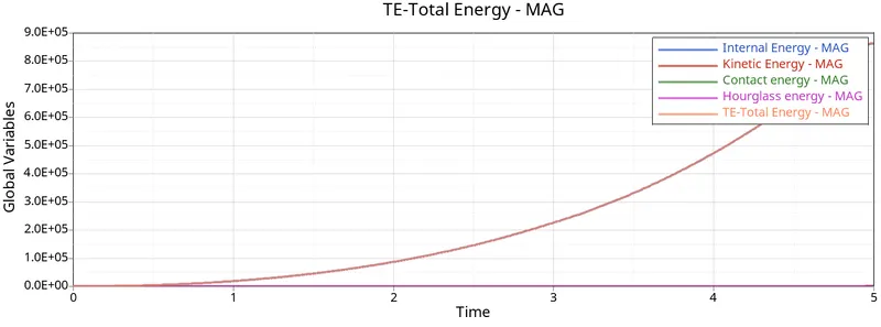
All Energies:

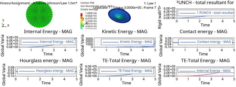
Processed Models:

 

Case 6 - LAW 27 (file - LAW27_0000.rad) with recommended shell properties:

• Here change the material card to LAW27 and change the shell properties to the recommended shell peroperties.
• It is an isotropic elastoplastic jhonson cook material model with an orthographic brittle failure model.

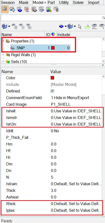
• Now change the parameters which is shown below.

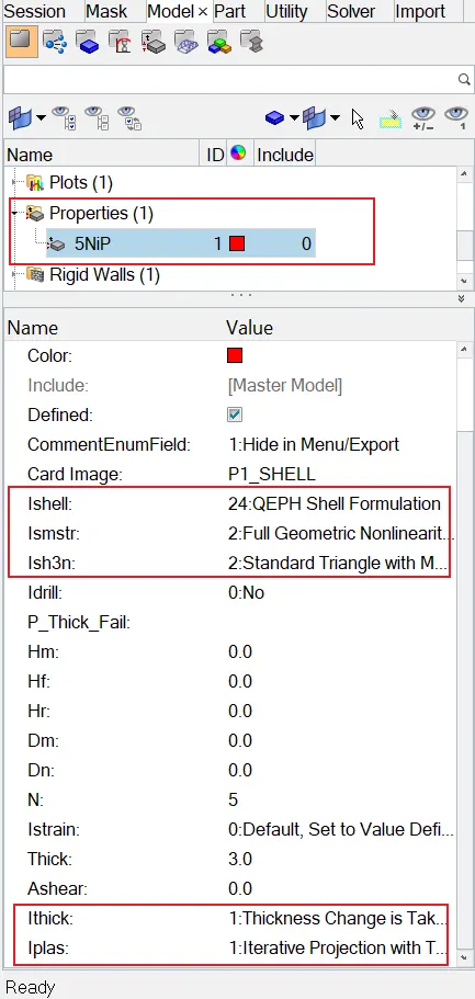
• Now run the simulation using radioss, the animation and TH files will be obtained in a required location which is shown below.

 

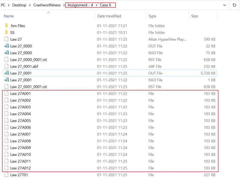
• Now go and open the 00001.out file with notepad.
• The obtained values for Energy Error,Mass Error,Internal Energy Error,Kinetic Energy Error and Contact Energy Error has been shown below.

 

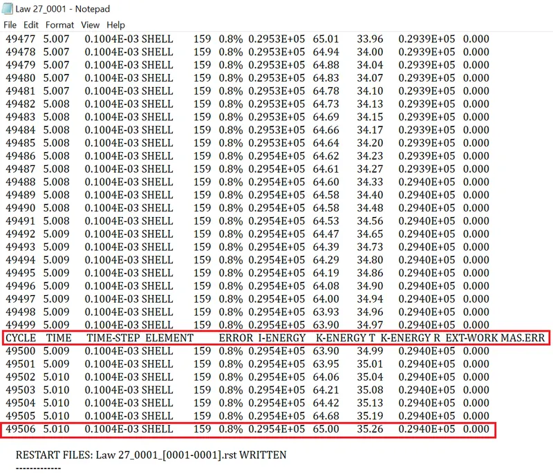
• The values obtained for this cycle are

• Energy Error - 0.8%
• Internal Energy - 0.2954E+05
• Kinetic Energy - 65
• External Work - 0.2940E+05
• Mass Error - 0
• Elapsed Time - 155.47s
• Total No of Cycles - 49506

Review the Simulation using HyperView:

• After completion of running the simulation,Switch to the hyperview.
• Open the appropriate .h3d file to review the simulation.
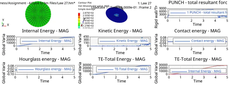
• The .h3d file is loaded and here the shell elements will be deleted due to brittleness which is shown below.

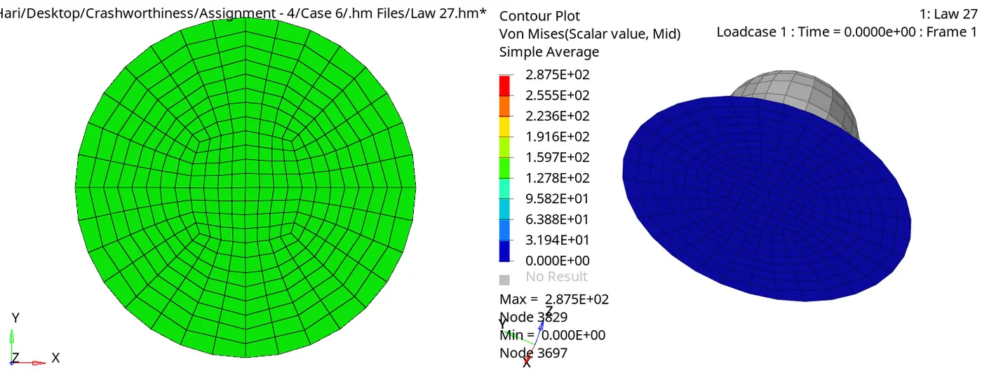
Plot the graphs using Hypergraph 2D:

• Now switch to the Hypergraph 2D and plot the graphs.

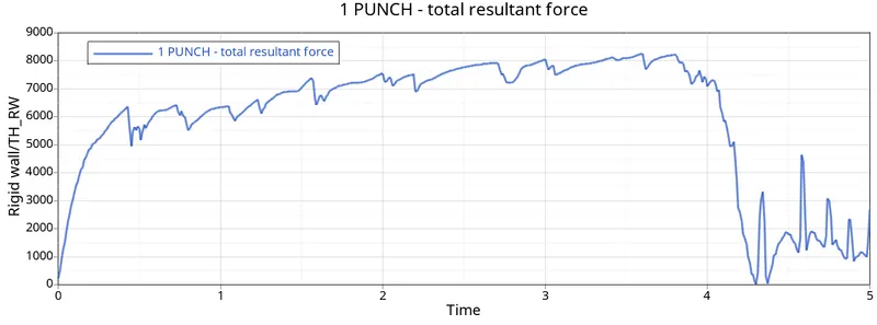
Rigid Wall Forces:

• The rigid wall forces starts increasing due to impact and decreases gradually,Because the elements are getting deleted and there will be no contact.
• The rigid wall forces graph obtained is shown below.

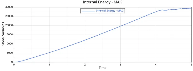
Internal Energy:

• Here the internal energy is similar to the previous case-3,The obtained internal energy graph is shown below.

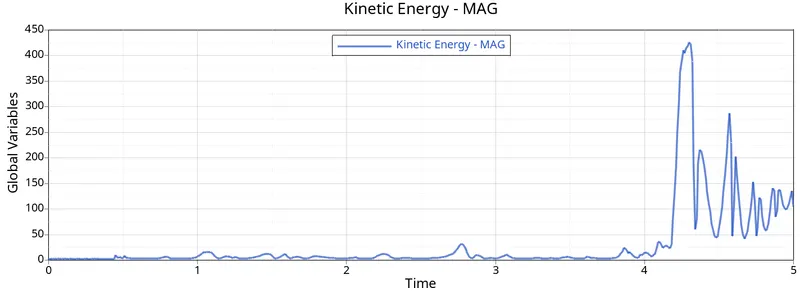
Kinetic Energy:

• Here the kinetic energy obtained is almost similar to the case-3 kinetic energy graph and the kinetic energy obtained is shown below.

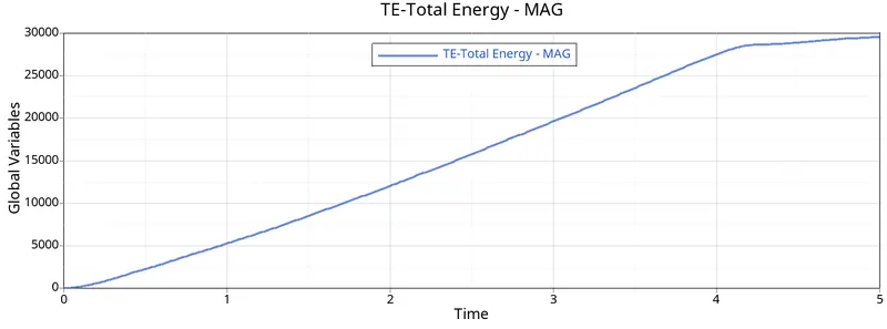
Total Energy:

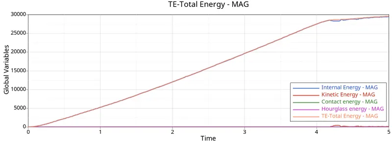
• The total energy increase with increase in internal energy and kinetic energy,The obtained total energy graph is shown below.

Hourglass and Contact Energy:

• Here hourglass energy is constant due to recommended parameters have been assigned.Here Ishell=24 QEPH is used,Due to this there is no houglass effect.
• Because the rigid ball is rigid body and the rupture plate is deformable body,So the contact energy is constant.
• If deformable bodies get in contact then only the contact energy increases.
• The obtained hourglass and contact energy graph is shown above.

All Energies:

Processed Models:

 

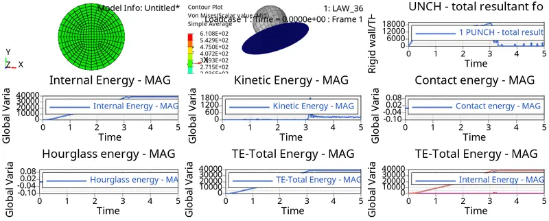
Case 7 - LAW 36 (file - LAW27_0000.rad) with recommended shell properties and given reference curve:

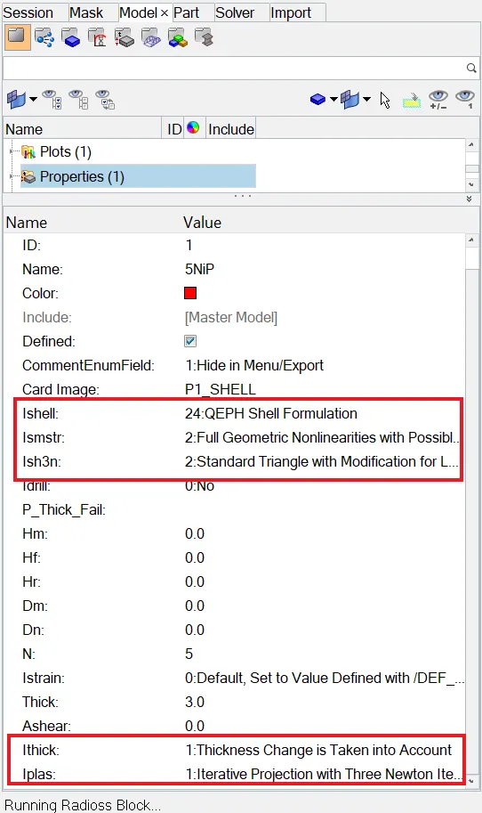
• Here change the material card to LAW36.
• A shell paremeters are changed to the recommended parameters.
• It's a elasto plastic piecewise linear material.

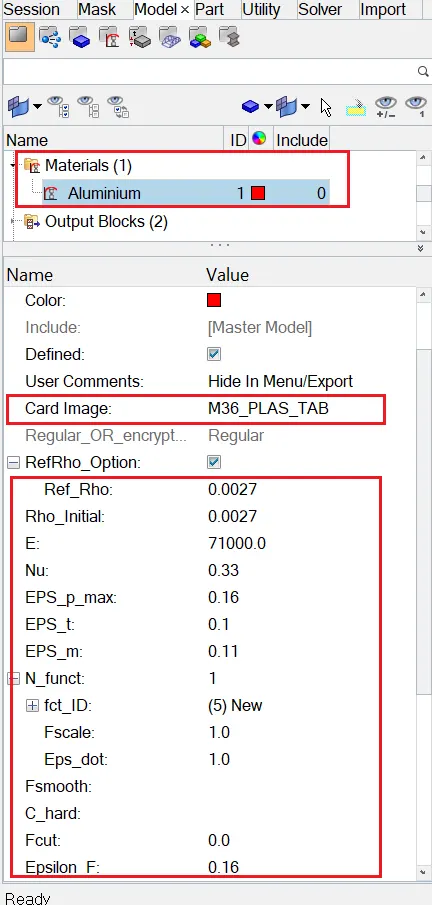
• After Defining the material card,We have to define a stress strain curve for this material.
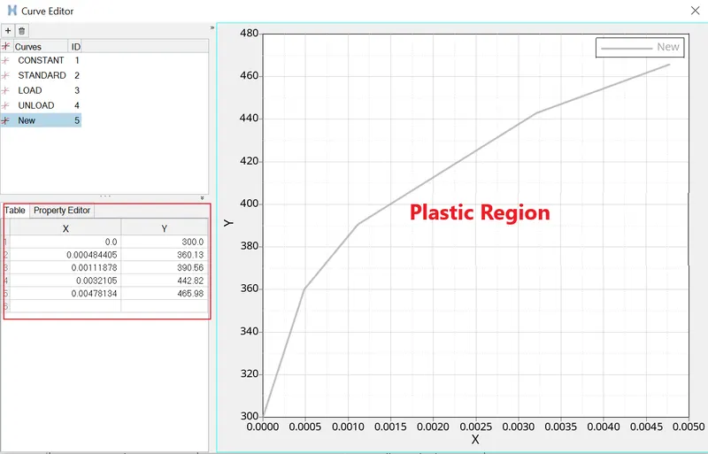
• We only want plastic region out of it,So we have to define a curve using given plastic strain and post-yield stress value manually.
• The curve will be defined based on the values given which is shown below.

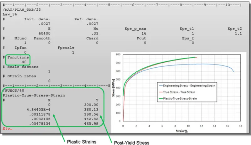
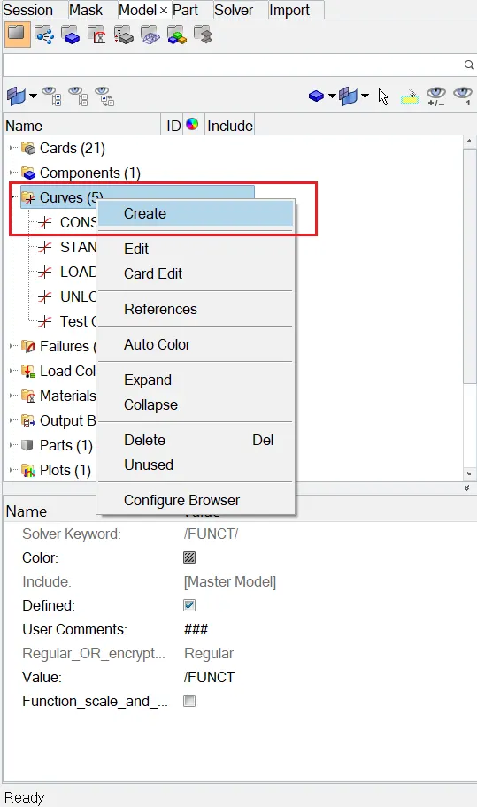
• To create a Curve, Right Click on the Model Browser ⟹ Create ⟹ Curve ⟹ Window Will Pop Up ⟹ Define a Curve using Platic Strains and Post-Yield Stress Values.

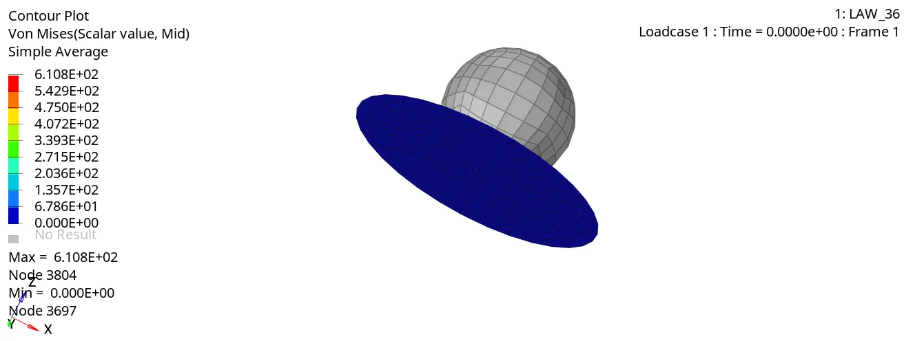
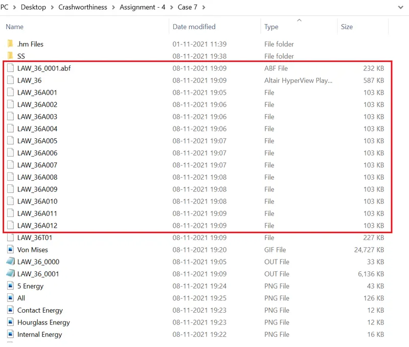
• Now run the simulation using radioss, the animation and TH files will be obtained in a required location which is shown below.

• Now go and open the 00001.out file with notepad.
• The obtained values for Energy Error, Mass Error, Internal Energy Error, Kinetic Energy Error and Contact Energy Error has been shown below.

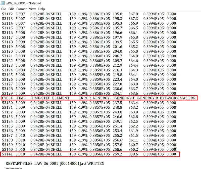
• The values obtained for this cycle are

• Energy Error - -1.9%
• Internal Energy - 0.3856E+05
• Kinetic Energy - 259.2
• External Work - 0.3994E+05
• Mass Error - 0
• Elapsed Time - 214.43 s
• Total No of Cycles - 53141

Review the Simulation using -HyperView:

• After completion of running the simulation,Switch to the hyperview.
• Open the appropriate .h3d file to review the simulation.
• The .h3d file is loaded and it is shown below.
• Here the shell elements will be deleted once it reaches maximum plastic strain which is shown below.
• Cause the material is assigned with both elastic and plastic.

Plot the graphs using-Hypergraph 2D:

• Now switch to the Hypergraph 2D and plot the graphs.
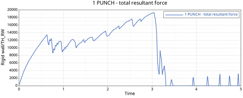
• The rigid wall forces graph is plotted which is shown below.

Rigid Wall Forces:

• Similarly as explained for the above Case-1. The graph obtained for the rigid wall forces is shown below.
• Here the elements are getting when it reaches maximum plastic strain.

Internal Energy:

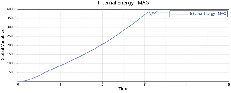
• The internal increases as same as in previous case.
• The obtained graph for internal energy is shown below.

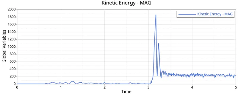
Kinetic Energy:

• The kinetic energy is somewhat similar to the Case - 5.
• The obtained kinetic energy graph is shown below.

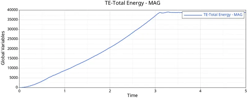
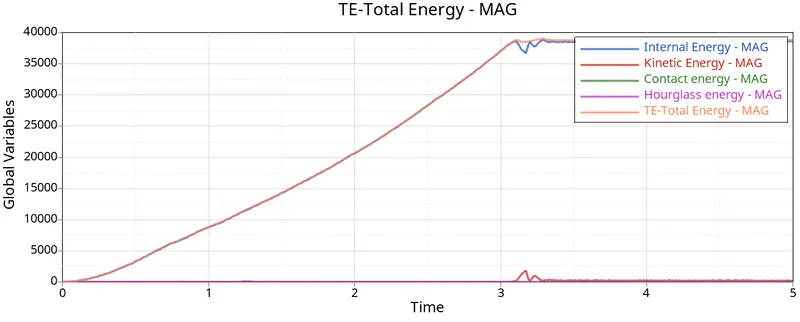
Total Energy:

• The total energy increases with increase in internal energy and kinetic energy.
• The obtained graoh for total energy is shown below.

 

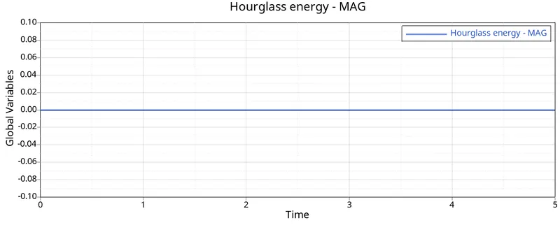
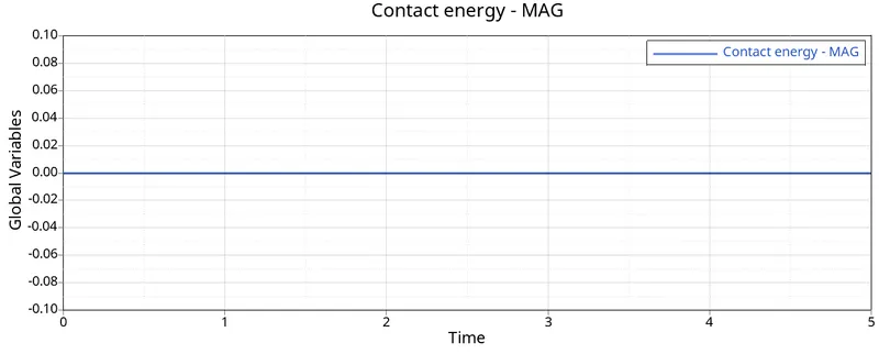
Hourglass and Contact Energy:

• Here hourglass energy is constant due to recommended parameters have been assigned.Here Ishell=24 QEPH is used,Due to this there is no houglass effect. Simillarly as same as for Case-7.
• Because the rigid ball is rigid body and the rupture plate is deformable body,So the contact energy is constant.
• If deformable bodies get in contact,then only the contact energy increases.
• The obtained hourglass and contact energy graph is shown below.

All Energy:

Processed models:

Comparison of all the 7 Cases:

Case	Energy Error	Internal Energy	Kinetic Energy	External work	Mass Error	Elapsed Time	Total No. of Cycles	Material Used	Changes in Material Parameters	Element Failure Behaviour
Case-1	0.8%	0.2730E+05	67.81	0.2721E+05	0	95.36s	49380	Jhonson-Cook [LAW2]	Used Default Shell Parameters and Run the Simulation	Elements Deleted
Case-2	4.1%	0.3082E+05	141.9	0.2980E+05	0	134.34s	49217	Jhonson-Cook [LAW2]	Changed the Values for Ifail_sh, Dadv, Ixfem in the Failure Card	Elements will be Cracked and Deleted
Case-3	0.8%	0.2744E+05	87.08	0.2736E+05	0	96.79 s	49407	Jhonson-Cook [LAW2]	Deleted the Failure Card from the Model Browser	Elements Deleted
Case-4	1.1%	0.3879E+05	3.931	0.3838E+05	0	131.47s	49303	Jhonson-Cook [LAW2]	Changed the Value for Maximum Plastic Strain [Eps_Max=0].	Elements Deformed, cracked but not Deleted
Case-5	7.4%	0.7195E+06	425.7	0.7780E+06	0	117.85s	47900	Elastic [LAW1]	Changed the Material Card to LAW1 and Kept the Same Material Properties.	Elements Deformed, Cracked but not Deleted
Case-6	0.8%	0.2954E+05	65	0.2940E+05	0	155.47s	49506	Elasto-Plastic-Brittle [LAW27]	Assigned the Rupture Parameters for the Plate and Used Recommended Element Parameters	Elements Deleted
Case-7	1.9%	0.3856E+05	259.2	0.3994E+05	0	214.43 s	53141	Elasto-Plastic-Tabulated [LAW36].	Created a Plastic Stress Strain Curve by Using Plastic Strains and Yield Stress Values.	Elements Deleted

Damage and Rupture Parameters:

• εpmax is the maximum plastic strain for element deletion for any loading (tensile , shear or compression).
• εt is the beginning of tensile damage. From this point the stress value defined in the curve is reduced by the factor.
• Where ε1 is the largest principal strain σ=σ[(ɛm−ɛ1)/(ɛm−ɛt)]
• εm is the end of the tensile damage. The stress value is null, but the element is not deleted.
• εf is the tensile failure strain value for element deletion.

Result:

• Hence the simulation for all the cases were carried out with different materials laws.
• Hence the simulation for all the cases were runned successfully.
• Hence the simulation for all the cases were reviewed by hyperview.
• Hence the graphs were plotted for all the  cases successfully.
• Finally compared all the results for those cases.

Conclusion:

• I conclude that LAW 36 is more suitable in real world testings as it shows the behaviour of Elasticity and Plasticity in real world.
• In this challenge, the learning outcomes are

1. The different materials cards and their behaviour.
2. The failure criteria for the material cards.
3. How the deformation is happening for the elements from material cards.
4. Damage and rupture parameters.
5. How to define a plastic region curve with plastic starin and post-yield stress values.