Assignment 4-RADIOSS Material Laws Challenge

Assignment 4-RADIOSS Material Laws Challenge

1. Aim

• Using the specified crash beam file, perform simulations on the mentioned scenarios.
• Analyze and compare the results obtained from all simulations and note down the mentioned points.

2. Objective

Objective 1: Perform the simulation as per the cases given below.

Case 1

•  Import the 'FAILURE_JOHNSON_0000.rad' file and run the model as it is. Give the title name 'Law2_epsmax_failure'.

Case 2

• Import the case 1 rad file, named 'Law2_epsmax_failure' and perform the simulation with failure plastic strain (EPS_p_max) and fail_Johson card enabled.
• Changes to be made in /FAIL/JOHNSON card:
• ifail_sh= 1
• Dadv= 1
• Ixfem= 1 
• Use the recommended values for the property card.
• Give the title name 'Law2_epsmax_crack'.

Case 3

• Import the case 2 rad file, named 'Law2_epsmax_crack' and perform the simulation by removing the fail_Johnson failure card. Give the title name 'Law2_epsmax_nofail'. 

Case 4 

• Import the case 3 rad file, named 'Law2_epsmax_nofail' and perform the simulation by removing both the failure plastic strain (EPS_p_max) and the fail_Jhonson failure card.

Case 5

• Import the case 4 rad file and perform the simulation by changing the material card to Law 1. Keep the same value for rho, E, and `nu` values.

Case 6 

• Import the case 1 rad file, named 'Law2_epsmax_failure' and perform the simulation with the law 36 material card.

  Fig 1: Properties For Materials (Case 6)

Case 7 

• Open the 'Law27_0000.rad' file and perform the simulation with the law 27 material card. Use the recommended shell properties.

Objective 2: Compare 7 cases as discussed in the last 3 slides, in a tabulated format based on:

• The Total number of cycles, Energy error, mass error, and simulation time.
• Notice the animation of all 5 and briefly describe the animations based on whether the elements are being deleted or cracked.
• Plot energies and notice any difference.
• Based on all the results, which case would represent the on-field scenario?
• Prepare a ppt/Docx and list the case-by-case results and your conclusion on why the failure happened.

3. Procedure

Case 1:

Step 1: Importing and opening the Model in Hyper Mesh RADIOSS

                   Initially, the beam file 'FAILURE_JOHNSON_0000.rad' is imported to hyper mesh through the solver deck. Save the file named 'Law2_epsmax_failure' by using Export > Solver Deck.

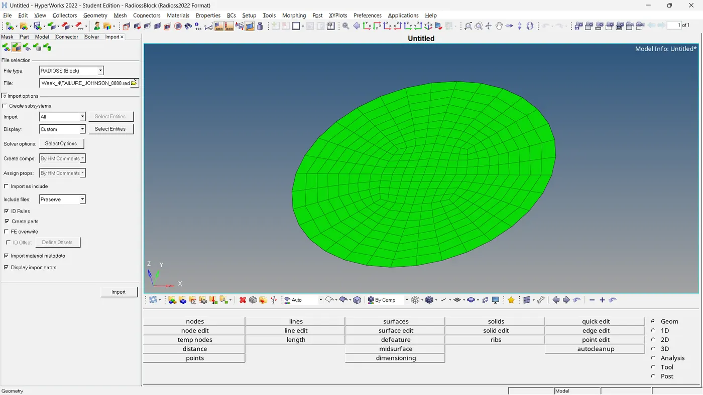
                                                     Fig 2: Importing The Model 'FAILURE_JOHNSON_0000.rad' Through Solver Deck (Case 1)

As per case 1, we have to simulate the model as it is. There are no changes to values such as shell properties, material properties, or failure models. Save the file named 'Law2_epsmax_failure'

For the model, The Run Time = 5.01 msec

                    Time-Frequency = 0.5 msec

 

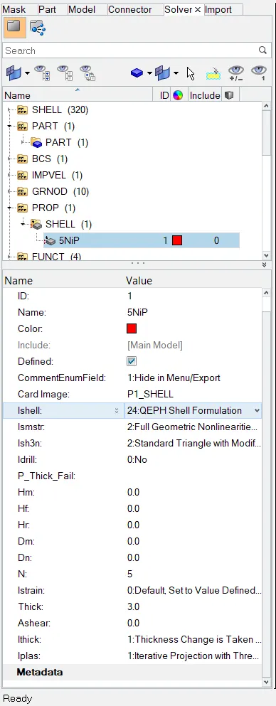
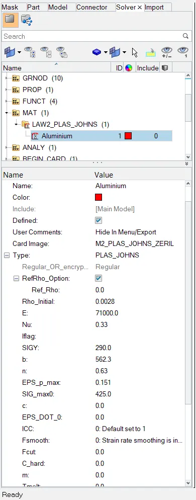
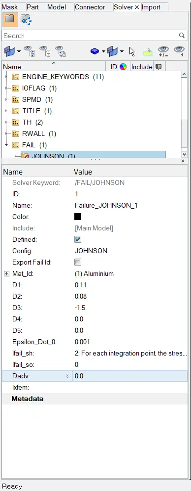
                                                                                      Fig 3: Default Shell, Material and Failure Properties (Case 1)

Step 2: Simulate the Model and Analysis of the Results

                             The simulation is done by following,

• Analysis >> Radioss >> Browse Input File Location >> Option = -nt 4 (No. Of Threads) >> Radioss 

After the simulation, save the file named 'Law2_epsmax_failure' by using Export > Solver Deck.

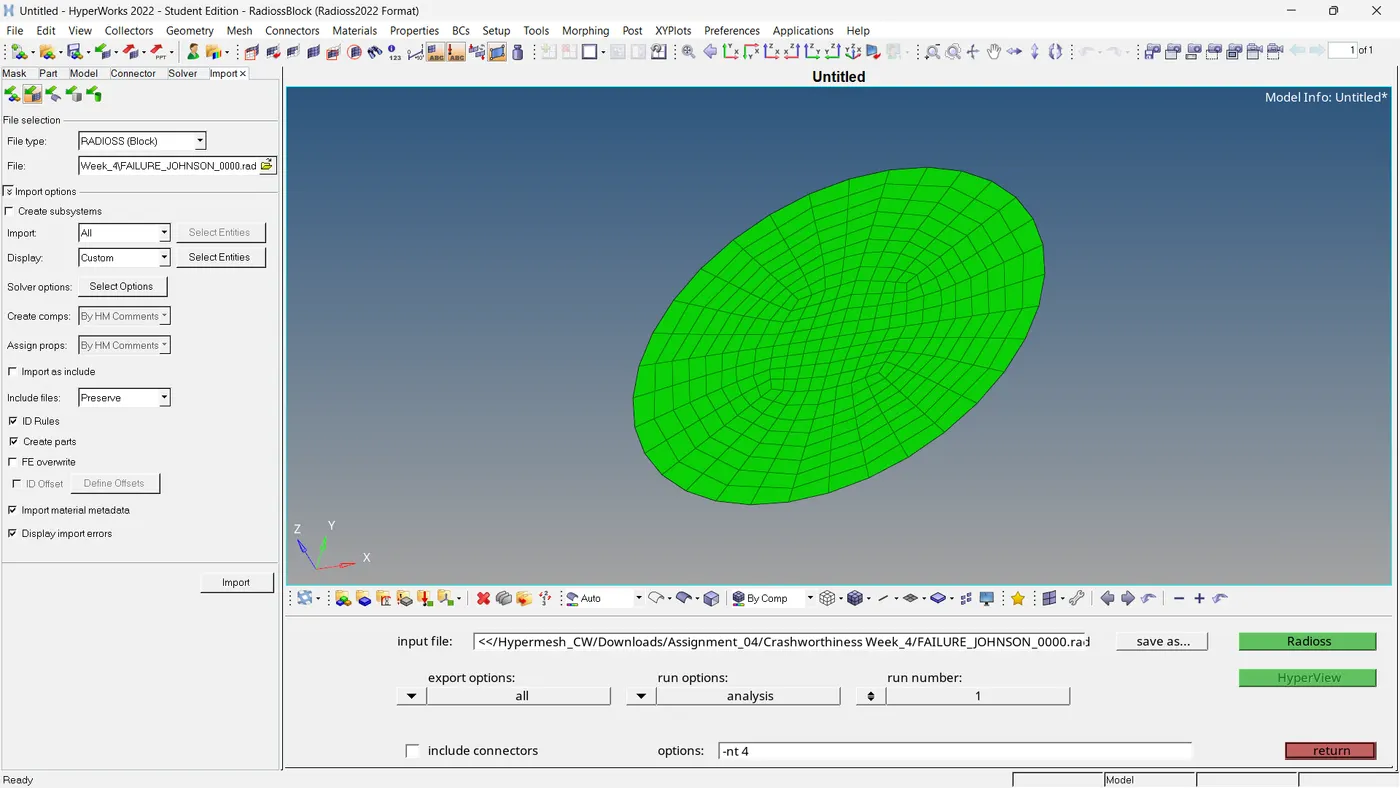
                                                                                               Fig 3: Loading Simulation Using Hyper Mesh (Case 1)

After the simulation, a job summary will pop up and it gives whether the simulation is completed or not. After a successful simulation, we can inspect the animations (.h3d file) through the hyper view. The output file includes the Energy Error, Mass Error, Energy Values, Mass Addition, etc. can be viewed by

• View >> Output File

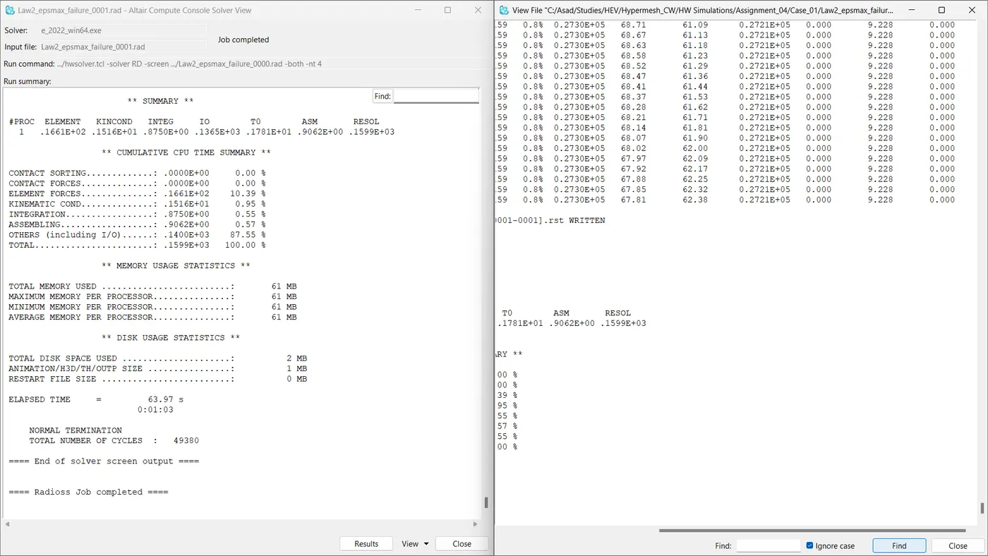
                                                                                          Fig 4:  Job Summary And Engine Output File (Case 1)

Using the hyper view, we can make the contours with Von Mises Stress. 

• Contours >> Result Type = Von Mises (S) >> Averaging Method = Simple >> Apply

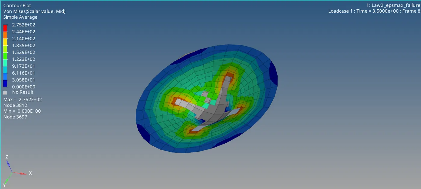
                                                                                               Fig 5: Contours- Von Mises Stress (Case 1)

 From the output file, 

1. Energy Error           = 0.8% 
2. Mass Error              = 0.0% 
3. Engine Run Time    = 63.97 Sec
4. Total No. Of Cycles = 49380

The errors are within the acceptable range. So we can continue with the model.

Step 3: Plotting Necessary Graphs Using Hyper Graph 2D

The plots are drawn using the hypergraph 2D, by opening the Time History File of the model and it can be used for the comparison between other cases. 

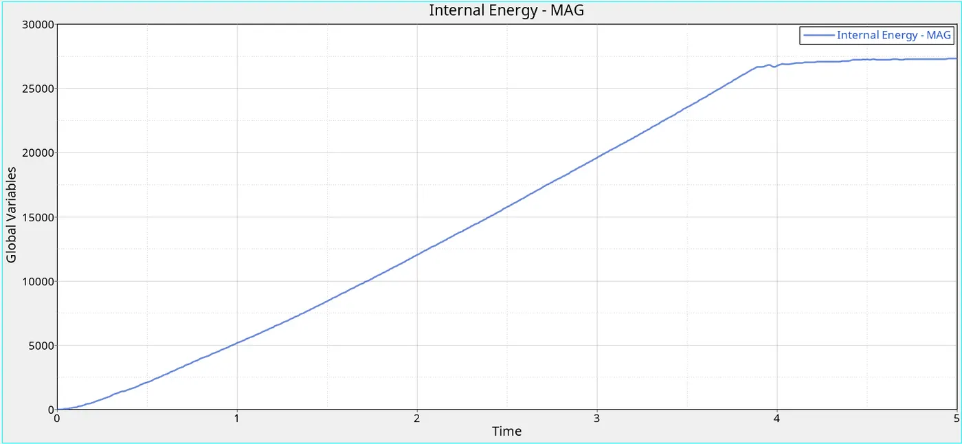
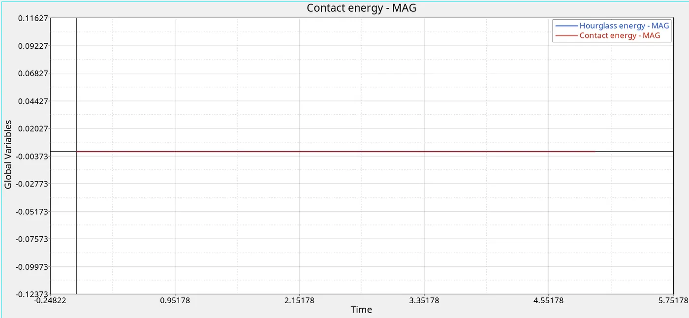
                                       Plot 1: Time Vs Internal Energy (Case 1)                                                      Plot 2: Time Vs Contact Energy, Hourglass Energy (Case 1)

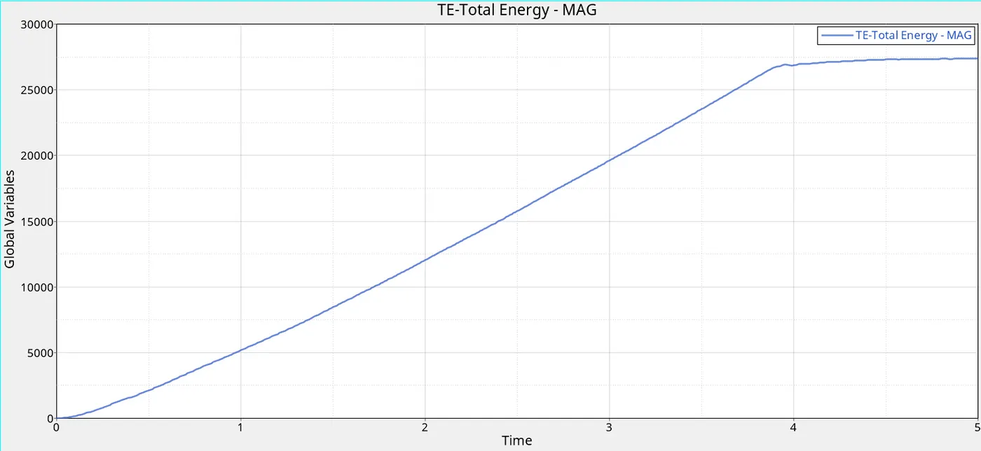
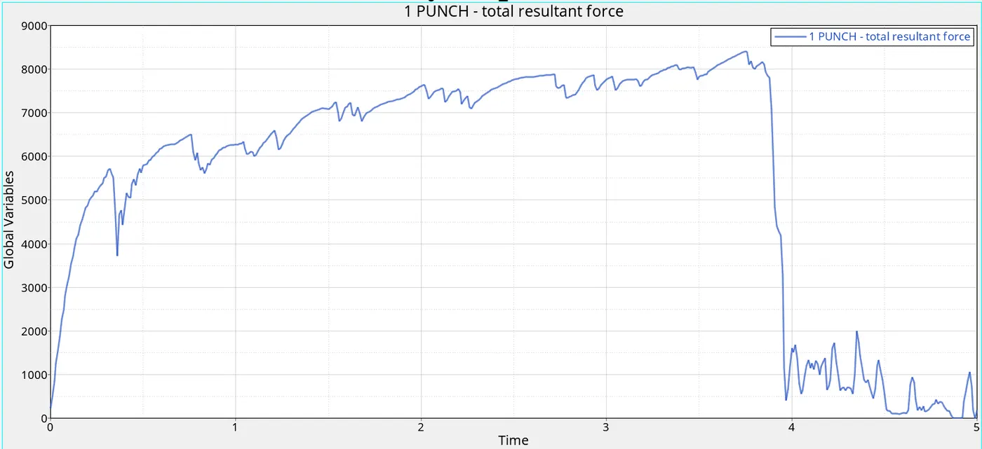
                                  Plot 3: Time Vs Total Energy (Case 1)                                                                    Plot 4: Time Vs Total Resultant Forces (Case 1)

Case 2

Step 1: Importing and opening the Model in Hyper Mesh RADIOSS

                                           Here is the starter file as the result file of case 1, 'Law2_epsmax_failure_0000.rad'. Here the goal is to modify the failure card and analyse the changes in the result. All other values like Shell and Material Properties remain the same. The values for the failure card are 

• ifail_sh= 1
• Dadv= 1
• Ixfem= 1 

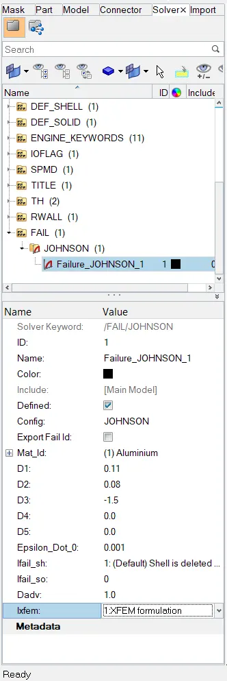
         Fig 6: Failure Card Editing (Case 2)

Step 2: Simulate the Model and Analysis of the Results

                                            After that, run the simulation and save the file named 'Law2_epsmax_crack_0000.rad'. By following previous methods, analyse the output file, and animations using Hyper View. 

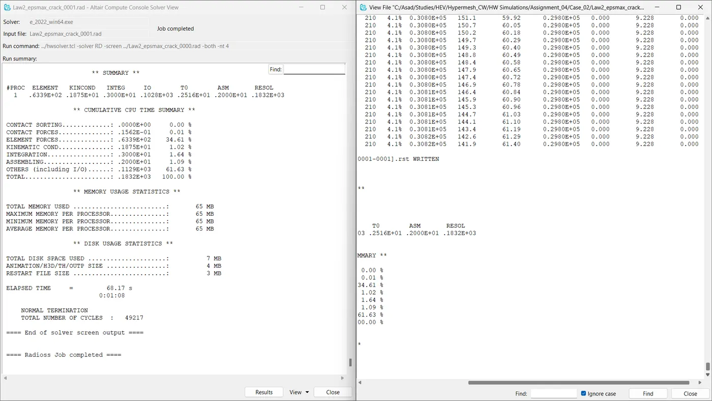
                                                                                          Fig 7: Job Summary And Engine Output File (Case 2)

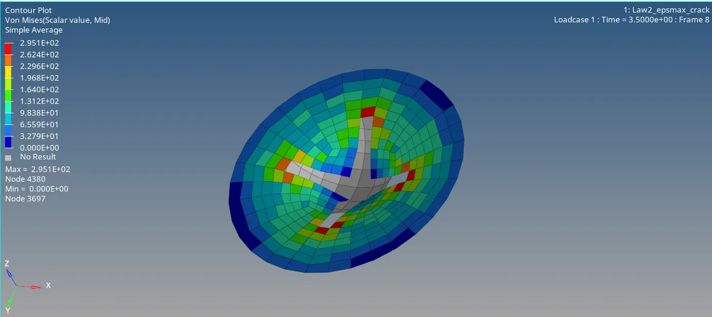
                                                                                               Fig 8: Contours- Von Mises Stress (Case 2)

From the output file, 

1. Energy Error           = 4.1% 
2. Mass Error              = 0.0% 
3. Engine Run Time    = 68.17 Sec
4. Total No. Of Cycles = 49217

The errors are within the acceptable range. So we can continue with the model.

Step 3: Plotting Necessary Graphs Using Hyper Graph 2D

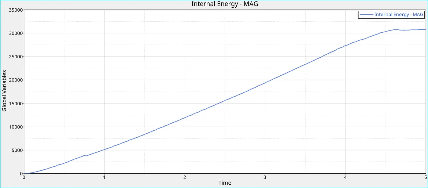
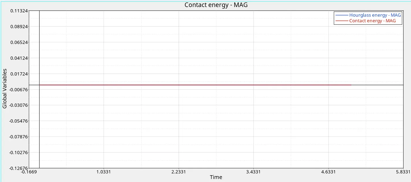
                                     Plot 5: Time Vs Internal Energy (Case 2)                                                      Plot 6: Time Vs Contact Energy, Hourglass Energy (Case 2)

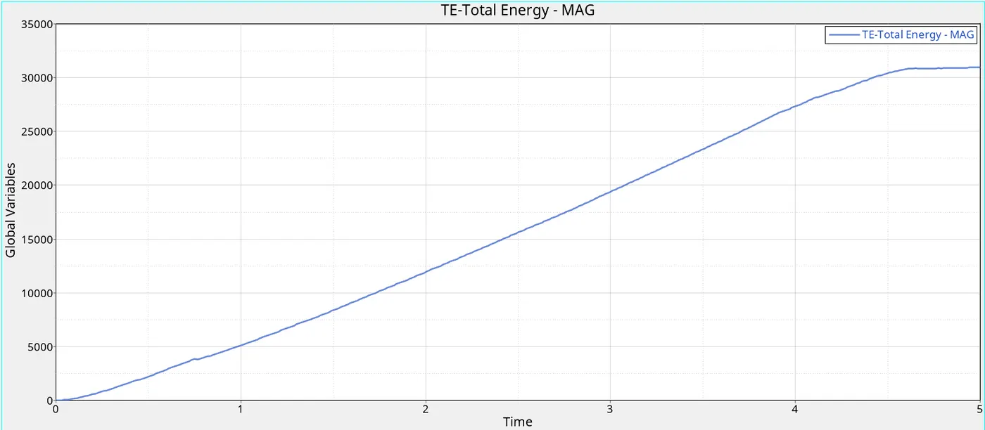
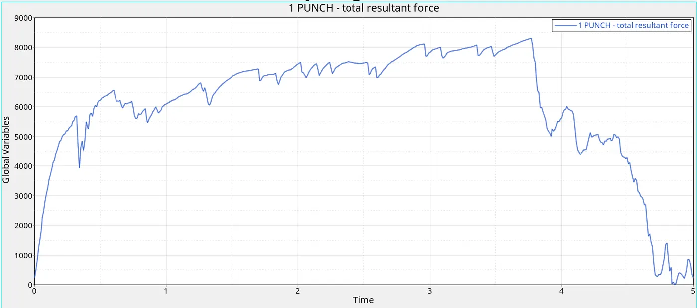
                                  Plot 7: Time Vs Total Energy (Case 2)                                                                    Plot 8: Time Vs Total Resultant Forces (Case 2)

Case 3

Step 1: Importing and opening the Model in Hyper Mesh RADIOSS

                                           Here is the starter file as the result file of case 2, 'Law2_epsmax_crack_0000.rad'. Here the goal is to remove the failure card and analyse the changes in the result. All other values like Shell and Material Properties remain the same. 

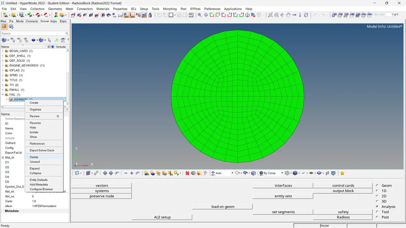
                                                                                                           Fig 9: Removing Failure Card (Case 3)

Step 2: Simulate the Model and Analysis of the Results

                                            After that, run the simulation and save the file named 'Law2_epsmax_nofail'. By following previous methods, analyse the output file, and animations using Hyper View. 

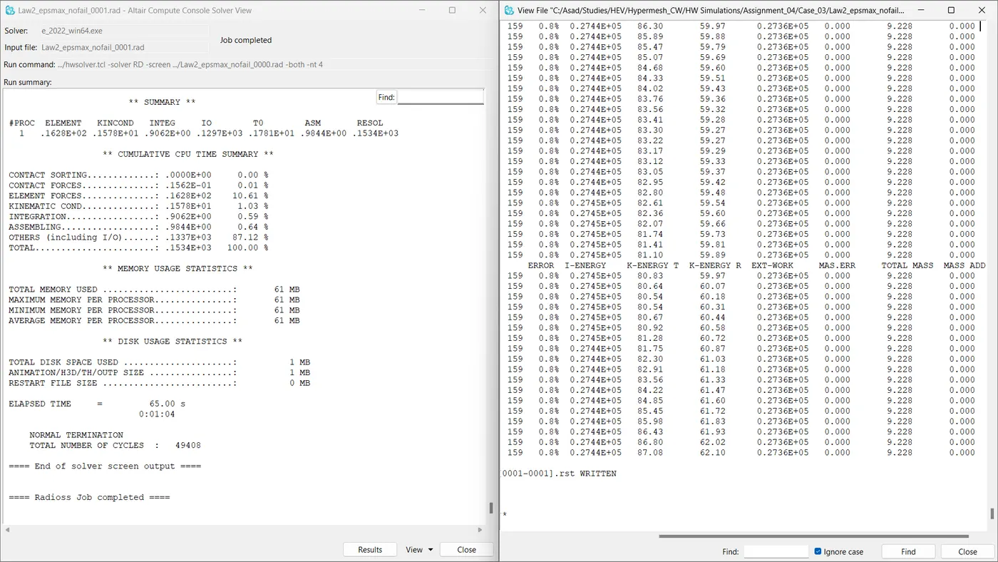
                                                                                          Fig 10: Job Summary And Engine Output File (Case 3)

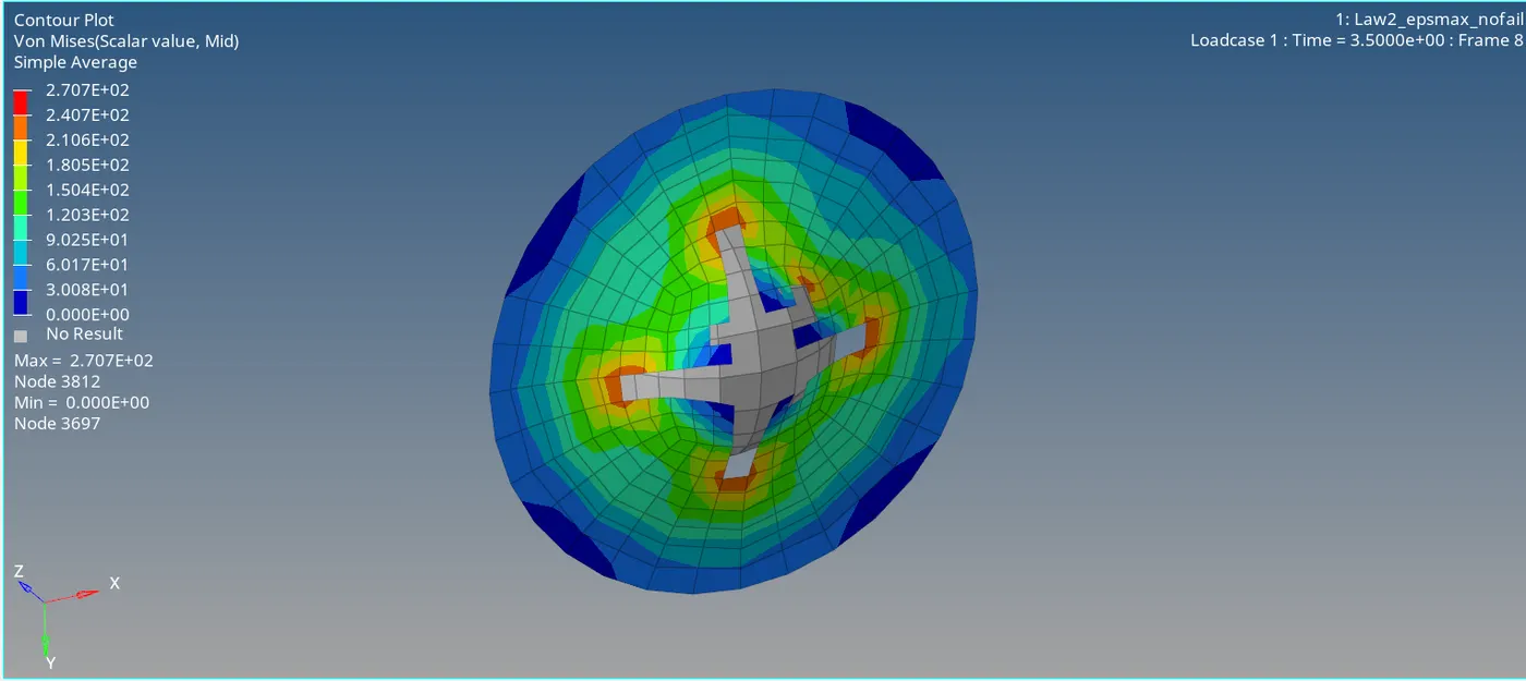
                                                                                               Fig 11: Contours- Von Mises Stress (Case 3)

From the output file, 

1. Energy Error           = 0.8% 
2. Mass Error              = 0.0% 
3. Engine Run Time    = 65.00 Sec
4. Total No. Of Cycles = 49408

The errors are within the acceptable range. So we can continue with the model.

Step 3: Plotting Necessary Graphs Using Hyper Graph 2D

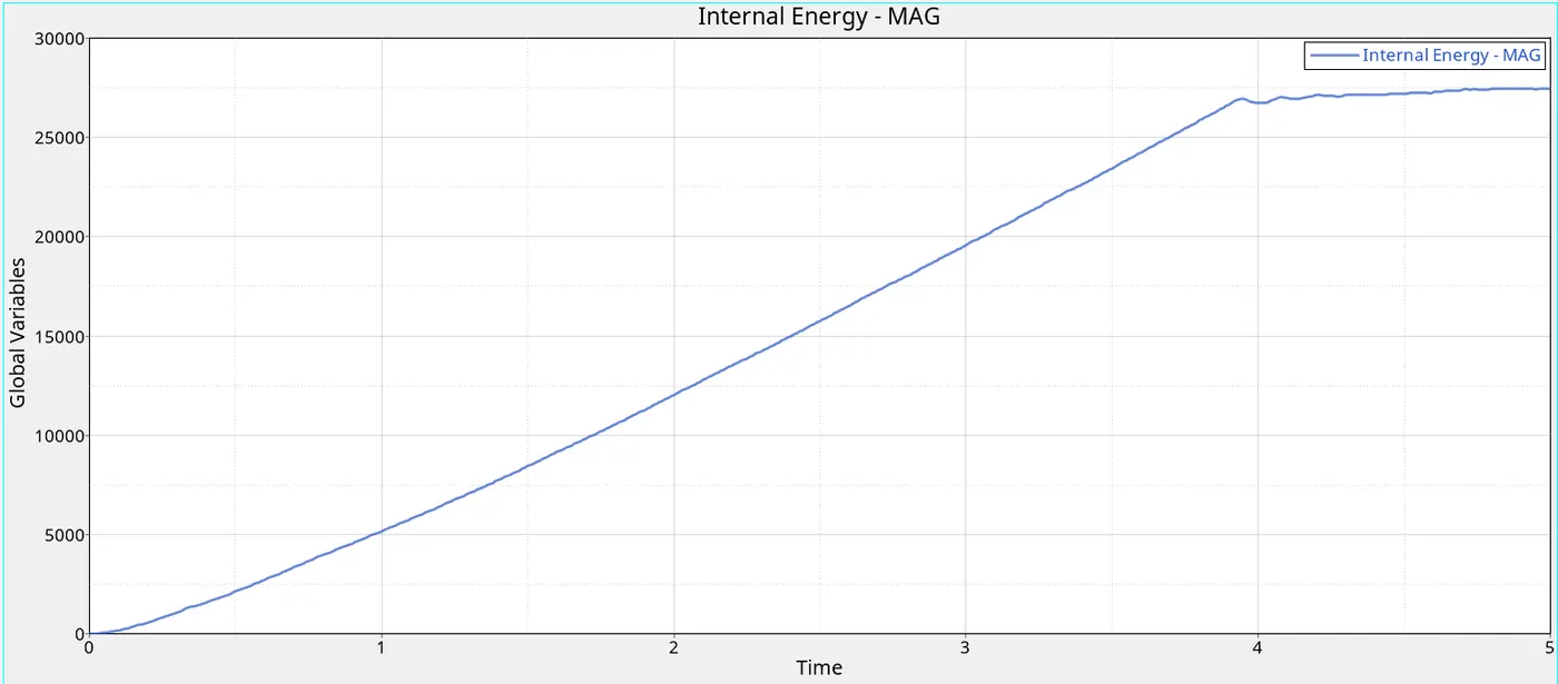
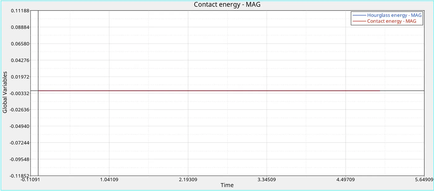
                                     Plot 9: Time Vs Internal Energy (Case 3)                                                      Plot 10: Time Vs Contact Energy, Hourglass Energy (Case 3)

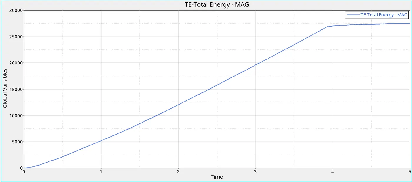
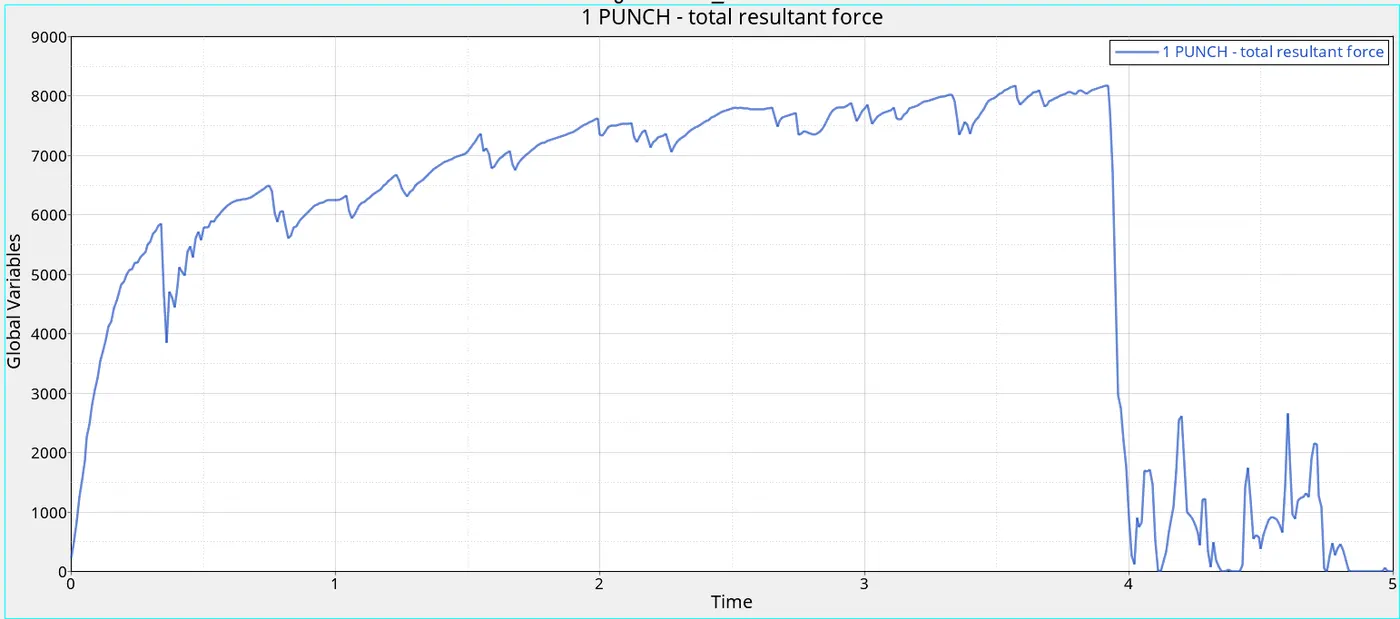
                                  Plot 11: Time Vs Total Energy (Case 3)                                                                    Plot 12: Time Vs Total Resultant Forces (Case 3)

Case 4

Step 1: Importing and Opening the Model in Hyper Mesh RADIOSS

                                           Here is the starter file as the result file of case 3, 'Law2_epsmax_nofail_0000.rad'. Here the goal is to remove both the failure plastic strain (EPS_p_max) and the fail_Jhonson failure card and analyse the changes in the result. All other values like Shell and Material Properties remain the same. 

The fail_Jhonson failure card is already removed from the file, and to remove the failure plastic strain, we have to change the value of (EPS_p_max) = 0. The changes are done in the material card using the solver browser.

     

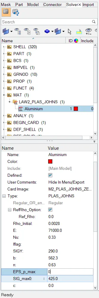
Fig 12: Failure Plastic Strain (EPS_p_max) Editing (Case 4)

Step 2: Simulate the Model and Analysis of the Results

                                            After that, run the simulation and save the file named 'Law2_noepsmax_nofail'. By following previous methods, analyse the output file, and animations using Hyper View. 

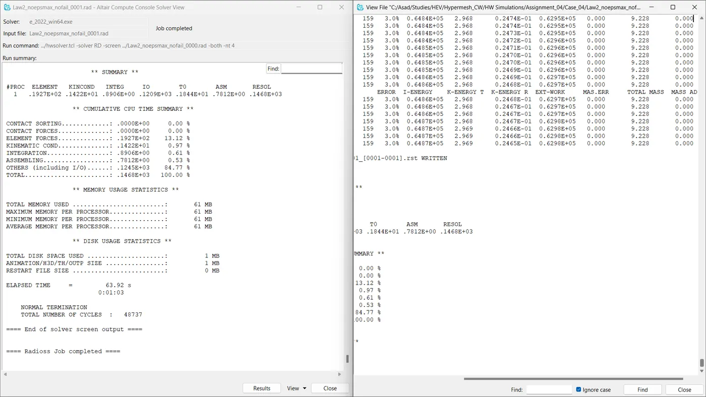
                                                                                          Fig 14: Job Summary And Engine Output File (Case 4)

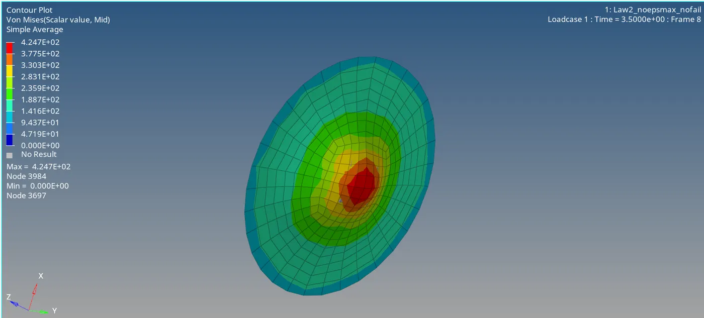
                                                                                               Fig 15: Contours- Von Mises Stress (Case 4)

From the output file, 

1. Energy Error           = 3.0% 
2. Mass Error              = 0.0% 
3. Engine Run Time    = 63.92 Sec
4. Total No. Of Cycles = 48737

The errors are within the acceptable range. So we can continue with the model.

Step 3: Plotting Necessary Graphs Using Hyper Graph 2D

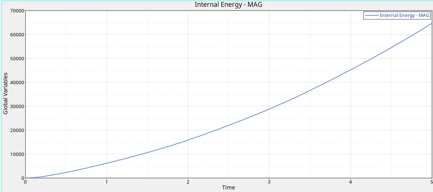
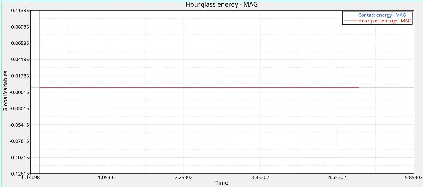
                                     Plot 13: Time Vs Internal Energy (Case 4)                                                      Plot 14: Time Vs Contact Energy, Hourglass Energy (Case 4)

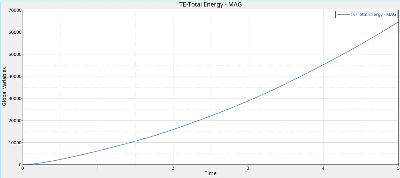
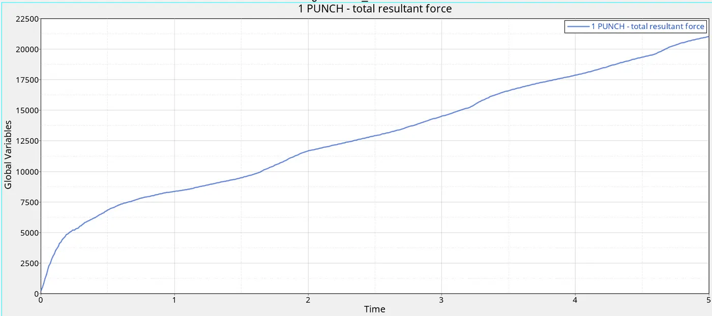
                                  Plot 15: Time Vs Total Energy (Case 4)                                                                    Plot 16: Time Vs Total Resultant Forces (Case 4)

Case 5

Step 1: Importing and Opening the Model in Hyper Mesh RADIOSS

                                       Here is the starter file as the result file of case 4, 'Law2_noepsmax_nofail_0000.rad'. By changing the material card to Law 1 (Linear Elastic Material), analyse the changes in the result.

To change the material to Law 1 and set the properties 

1. Rho_initial = 0.0028
2. E = 71000.00
3. nu = 0.33

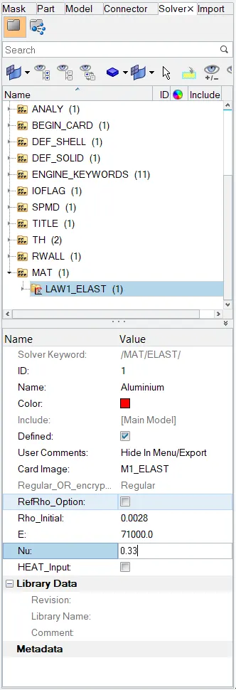
Fig 16: Material and Property Editing (Case 5)

Step 2: Simulate the Model and Analysis of the Results

                                            After that, run the simulation and save the file named 'Law1_noepsmax_nofail'. By following previous methods, analyse the output file, and animations using Hyper View. 

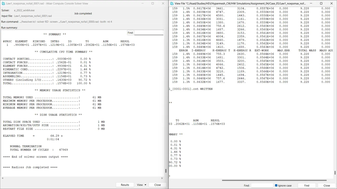
                                                                                          Fig 17: Job Summary And Engine Output File (Case 5)

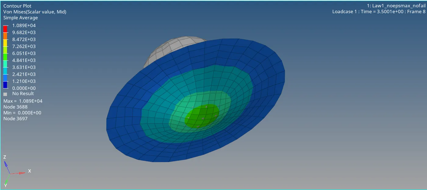
                                                                                               Fig 18: Contours- Von Mises Stress (Case 5)

From the output file, 

1. Energy Error           = 1.3% 
2. Mass Error              = 0.0% 
3. Engine Run Time    = 64.29 Sec
4. Total No. Of Cycles = 47969

The errors are within the acceptable range. So we can continue with the model.

Step 3: Plotting Necessary Graphs Using Hyper Graph 2D

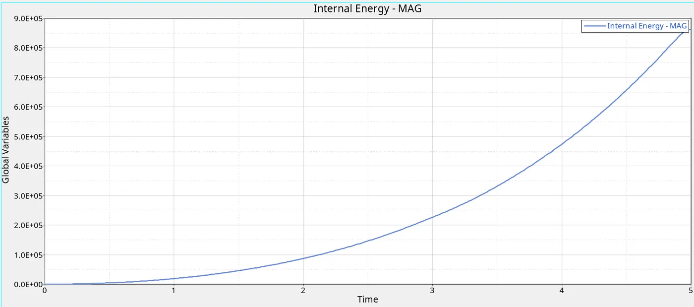
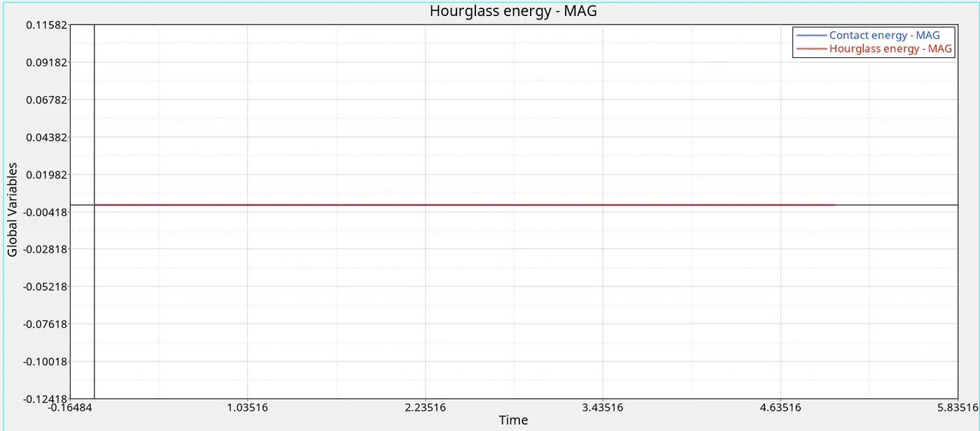
                                     Plot 17: Time Vs Internal Energy (Case 5)                                                      Plot 18: Time Vs Contact Energy, Hourglass Energy (Case 5)

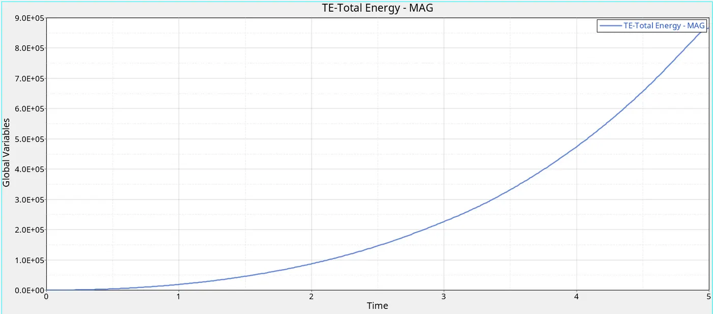
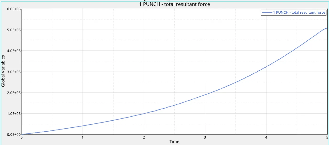
                                  Plot 19: Time Vs Total Energy (Case 5)                                                                    Plot 20: Time Vs Total Resultant Forces (Case 5)

Case 6

Step 1: Importing and Opening the Model in Hyper Mesh RADIOSS

                                  Here is the starter file as the result file of case 1, 'Law2_epsmax_failure_0000.rad'. By changing the material card to Law 36, analyse the changes in the result.

To change the material to Law 36 and set the properties. 

The Law 36 material needs a curve, and the curve is created using the mentioned co. ordinates, (Refer Video: Material 7) 

X	Y
0	300
4.84405E-4	360.13
0.00111878	390.56
0.0032105	442.82
0.00478134	465.95

       Table 1: Coordinates For Law36 Curve

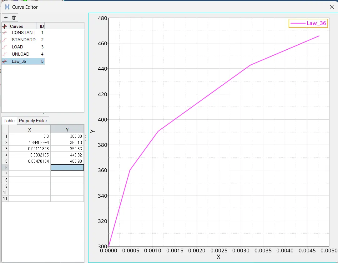
                                                                                                            Fig 19: Curve For Law36 Material Properties

After that, the curve is to be assigned on the material card (fct_Id), and other properties are shown in the objectives. 

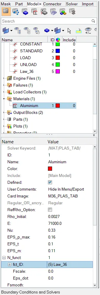
Fig 20: Material and Property Editing (Case 6)

Step 2: Simulate the Model and Analysis of the Results

                                            After that, run the simulation and save the file named 'Law36_epsmax_failure_0000.rad'. By following previous methods, analyse the output file, and animations using Hyper View.

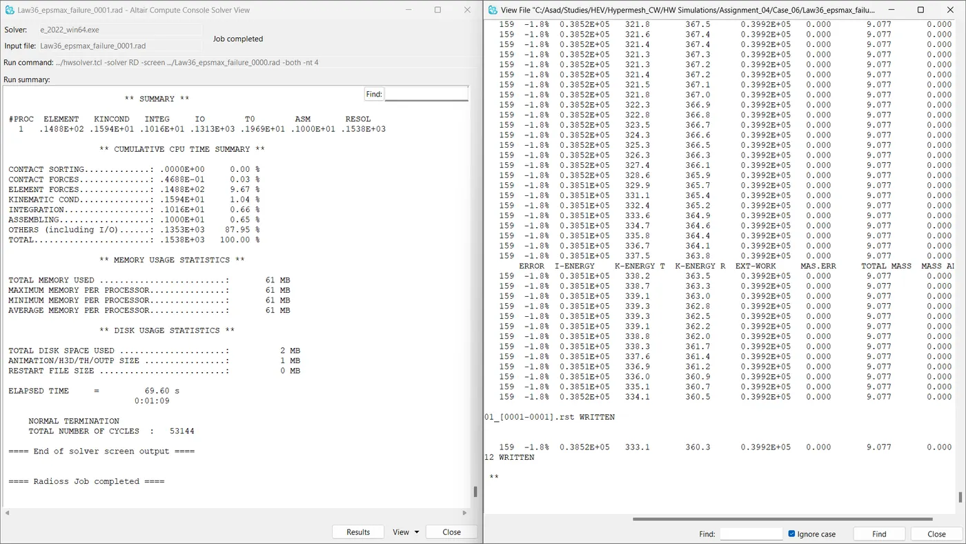
                                                                                           Fig 21: Job Summary And Engine Output File (Case 6)

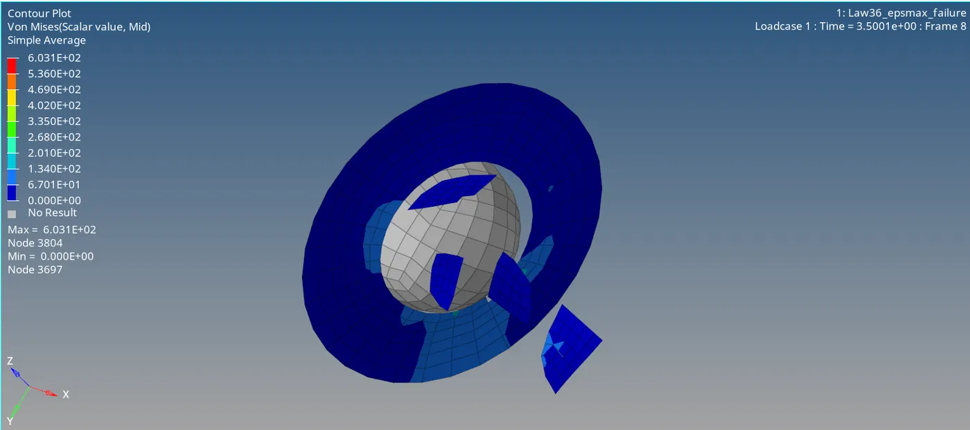
                                                                                             Fig 22: Contours- Von Mises Stress (Case 6)

From the output file, 

1. Energy Error           = -1.8% 
2. Mass Error              = 0.0% 
3. Engine Run Time    = 67.00 Sec
4. Total No. Of Cycles = 53144

The errors are within the acceptable range. So we can continue with the model.

Step 3: Plotting Necessary Graphs Using Hyper Graph 2D

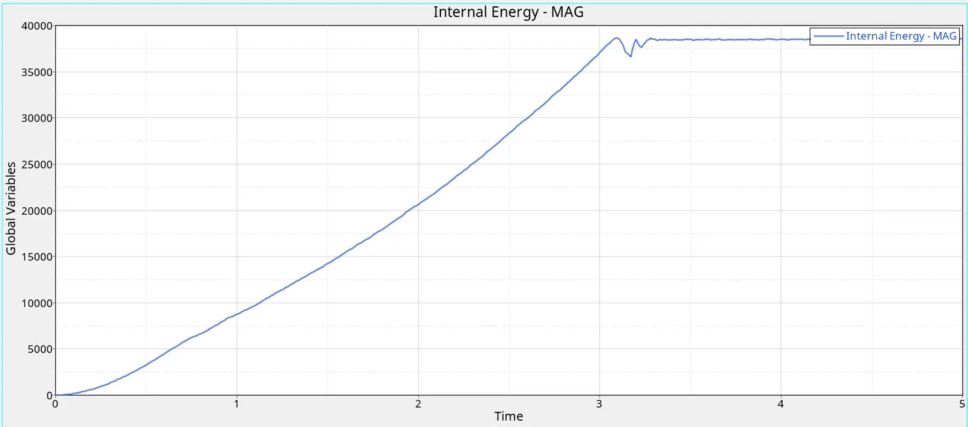
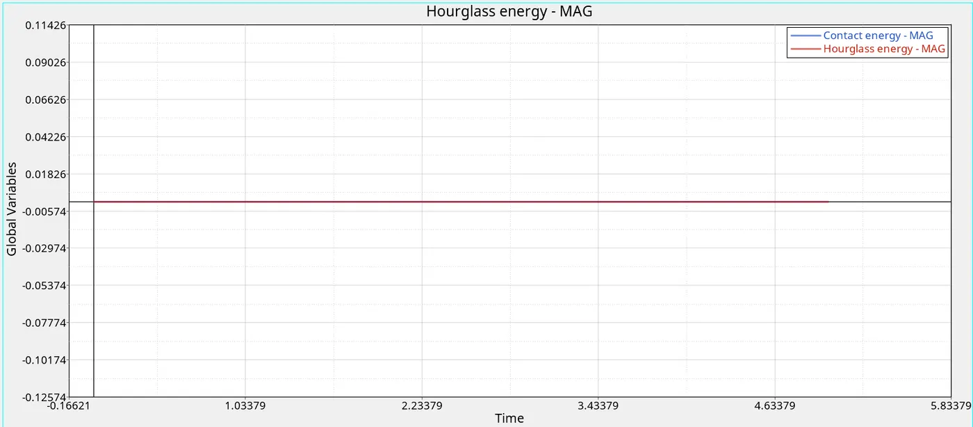
                                     Plot 21: Time Vs Internal Energy (Case 6)                                                            Plot 22: Time Vs Contact Energy, Hourglass Energy (Case 6)

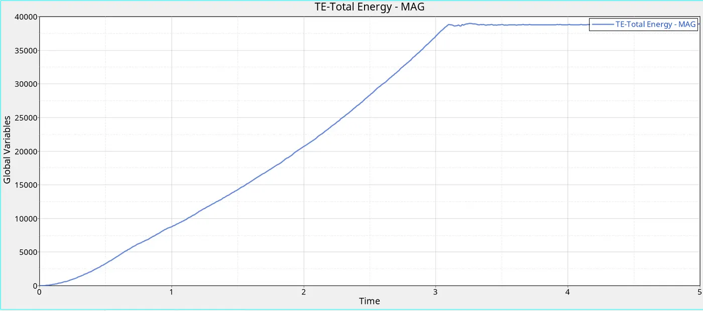
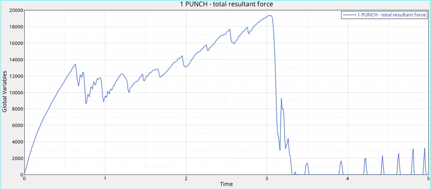
                                  Plot 23: Time Vs Total Energy (Case 6)                                                                              Plot 24: Time Vs Total Resultant Forces (Case 6)

Case 7

Step 1: Importing and Opening the Model in Hyper Mesh RADIOSS

                                                       Initially, the beam file 'Law27_0000.rad' is imported to hyper mesh through the solver deck. Change the material card to the law 27 material card. Use the recommended shell properties. The default shell element properties are

1. I_shell=24
2. I_smstr=2
3. I_sh3n=2
4. N=5
5. I_thick=1
6. I_plas=1

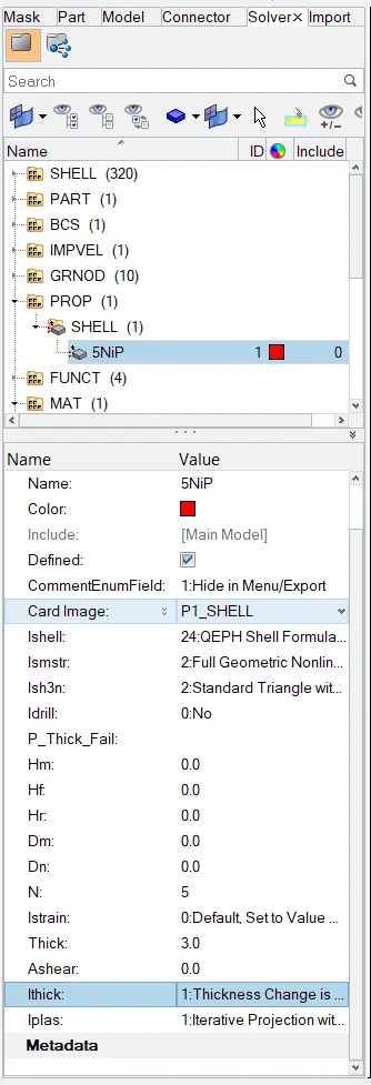
Fig 23: Material and Shell Property Editing (Case 7)

Step 2: Simulate the Model and Analysis of the Results

                                                 After that, run the simulation. By following previous methods, analyse the output file, and animations using Hyper View.

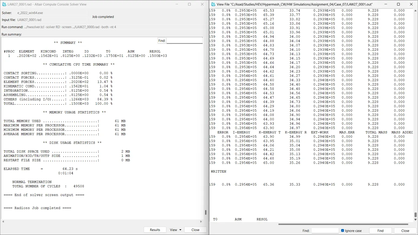
                                                                                           Fig 24: Job Summary And Engine Output File (Case 7)

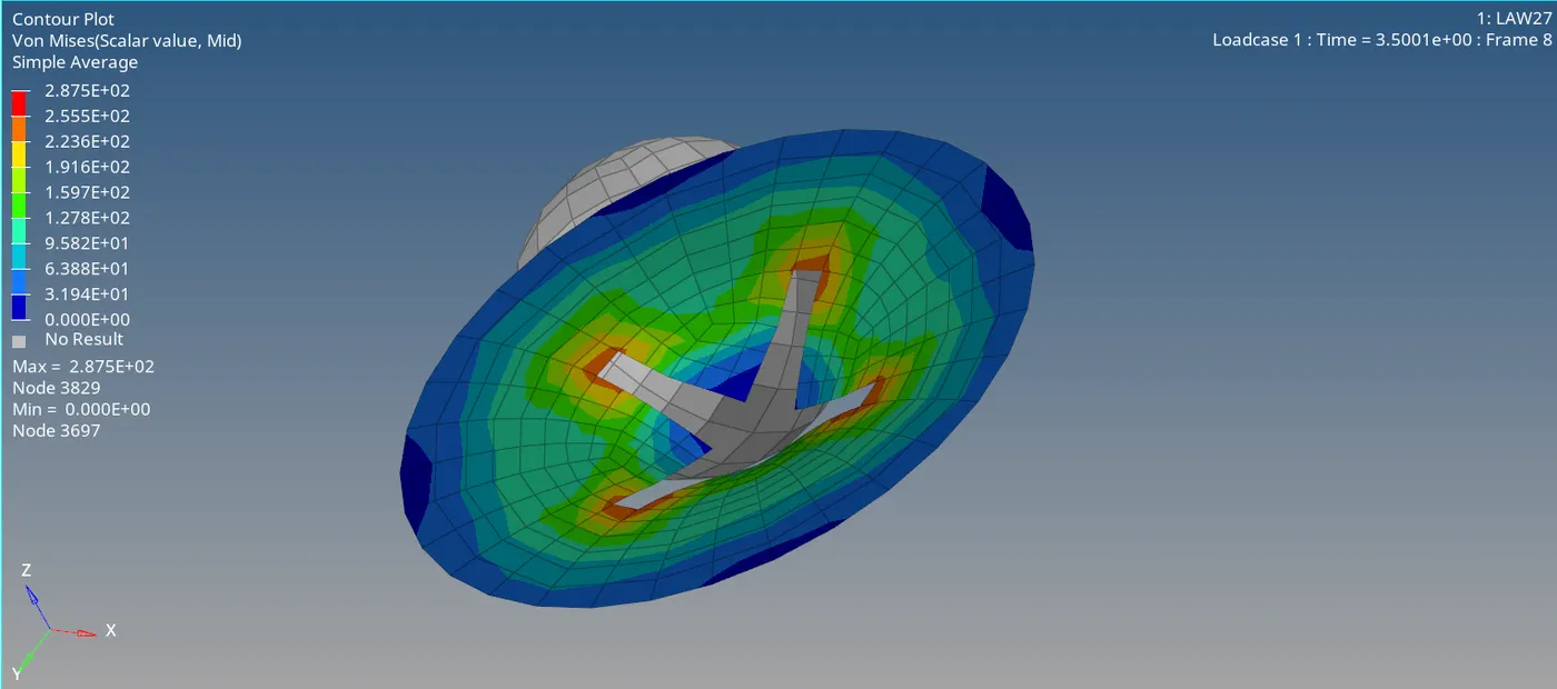
                                                                                             Fig 25: Contours- Von Mises Stress (Case 7)

From the output file, 

1. Energy Error            = 0.8% 
2. Mass Error               = 0.0% 
3. Engine Run Time     = 64.23 Sec
4. Total No. Of Cycles = 49508

The errors are within the acceptable range. So we can continue with the model.

Step 3: Plotting Necessary Graphs Using Hyper Graph 2D

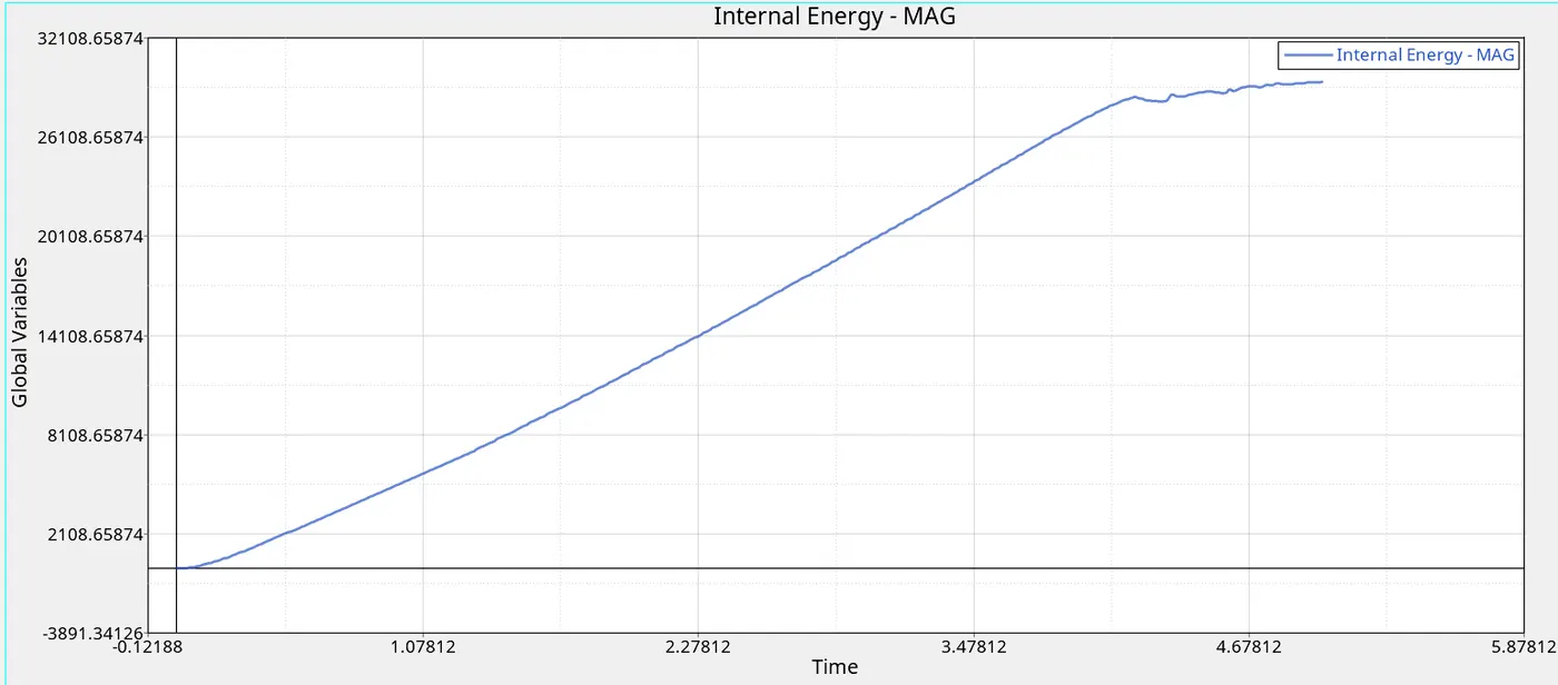
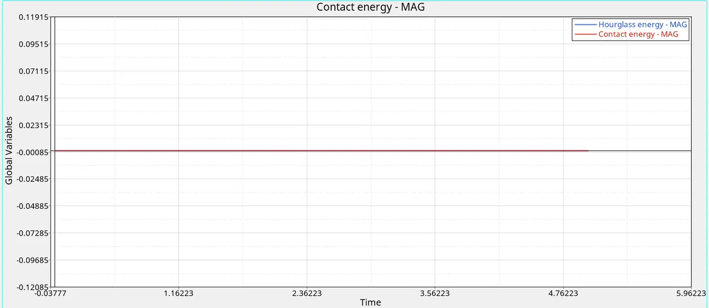
                                     Plot 25: Time Vs Internal Energy (Case 7)                                                      Plot 26: Time Vs Contact Energy, Hourglass Energy (Case 7)

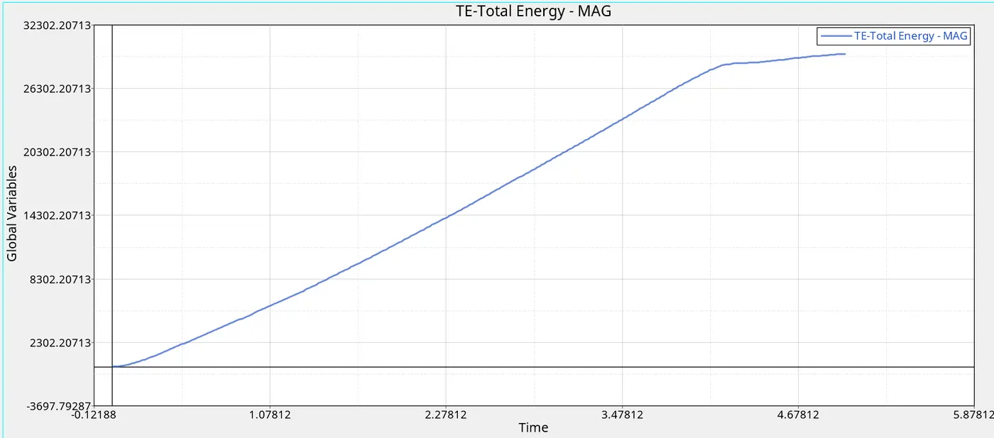
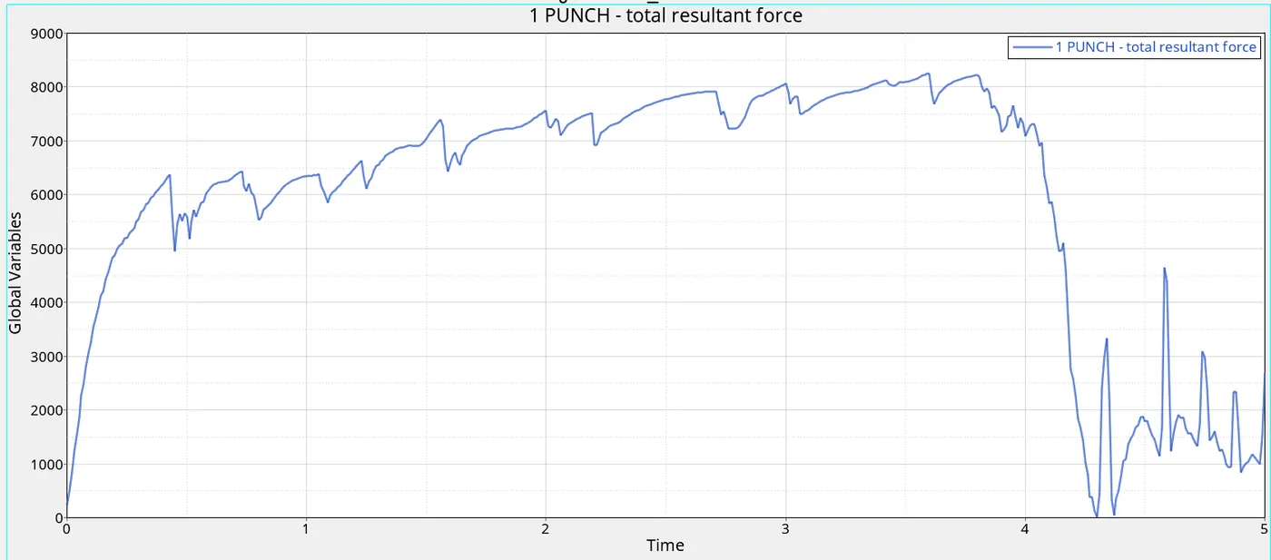
                                  Plot 27: Time Vs Total Energy (Case 7)                                                                       Plot 28: Time Vs Total Resultant Forces (Case 7)

4. Conclusions

          For an easy comparison, the results of each simulation are tabulated below.

No	Simulation Name/File Name	Material Law	Simulation Time	Total No. of Cycles	Energy Error	Mass Error	Maximum Stress (Acting Node No)	Element Observation
1	Law2_epsmax_failure	/MAT/LAW2/(PLAS_JOHNS)	63.97	49380	0.8	0.00	2.752E+2 (3812)	Elements get deleted
2	Law2_epsmax_crack	/MAT/LAW2/(PLAS_JOHNS)	68.17	49217	4.1	0.00	2.951E+2 (4380)	Elements get cracked and then they get deleted
3	Law2_epsmax_nofail	/MAT/LAW2/(PLAS_JOHNS)	65.00	49408	0.8	0.00	2.707E+2 (3812)	Element get deleted
4	Law2_noepsmax_nofail	/MAT/LAW2/(PLAS_JOHNS)	63.92	48737	3.0	0.00	4.247E+2 (3984)	Element not deleted
5	Law1_noepsmax_nofail	/MAT/LAW1/(ELAST)	64.29	47969	1.3	0.00	1.087E+4 (3688)	Element not deleted
6	Law36_epsmax_failure	/MAT/LAW36/(PLAS_TAB)	67.00	53144	-1.8	0.00	6.031E+2 (3804)	Elements get deleted
7	Law27_0000	/MAT/LAW27/(PLAS_BRIT)	64.23	49508	0.8	0.00	2.875E+2 (3829)	Elements get deleted

                                                                                                          Table 2: Comparison Of Simulation Results In Different Cases

4. Conclusions

Case 1

• In case 1, both the failure card 'failure_Johnson' and the values of EPS_p_max=0.151 are assigned to the model. For the EPS_p_max, it indicates that as soon as the element reaches 15.1% of plastic strain, the elements are deleted.  We can observe it from the simulation. 
• The internal energy and total energy gradually increase with time. The time comes when the elements start to delete, the increase in energy stops and the graphs take linear shapes
• The total resultant force curve has a sudden drop when the time is about 4ms, and finally, it reaches zero. It occurs when the collision and the element deletion occur in the simulation. 

Case 2

• In case 2, the values for the failure card are assigned. Ifail_sh is the Shell failure flag set to 1 which will generate a crack in the shell element when Ixfem is set to 1, Dadv is the criterion for the crack advancement. It leads to a crack developed on elements that exceed the plastic strain limit (EPS_p_max) and then it gets deleted. In the simulation, we can see the crack propagation through the elements.
• The internal energy and total energy gradually increase with time. The time comes when the elements start to delete, the increase in energy stops and the graphs take linear shapes
• The total resultant force curve has a gradual drop when the time is about 4ms, and finally, it reaches zero. It occurs because there is a crack formation before the collision and the element deletion occurs in the simulation. 

Case 3

• Here the failure card is deleted. So only the EPS_p_max value will be considered in element deletion. Because there is no failure card, there is no crack propagation. When the plastic strain reaches the limit the elements get deleted.
• The internal energy and total energy gradually increase with time. The time comes when the elements start to delete, the increase in energy stops and the graphs take linear shapes
• The total resultant force curve has an instantaneous drop when the time is about 4ms, and finally, it reaches zero. It occurs because as soon as the elements reach the limit, the element is directly deleted.

Case 4

• In this scene, both the failure card and EPS_p_max are deleted (Set to default=10^30 and it is high). So there are no limits for the element deletion. The elements are stretched until the maximum value of maximum stress reaches that is 4.247E+2. The elements do not get deleted in the simulation.
• The internal energy and total energy gradually increase with time. There is no drop in energy because there are no element deletions
• The total resultant force curve increases with time, and it never decreases or reaches zero. The reason is there are no element deletions throughout the simulation. 

Case 5

• Here the material is changed from '/MAT/LAW2/(PLAS_JOHNS)' to /MAT/LAW1/(ELAST). which has the properties of elastic material. Also, the failure card and EPS_p_max are deleted. There is no plastic region. the material can absorb a vast amount of energy without any cracks or element deletion. From the simulation, we can see that the maximum stress is 1.087E+4 which is way higher than other materials. Even with this much stress, the elements overcome the deletion or cracks because of the elastic property of the material.
• The internal energy and total energy gradually increase with time. There is no drop in energy because there are no element deletions
• Also, like in case 4, The total resultant force curve increases with time, and it never decreases or reaches zero. The reason is there are no element deletions throughout the simulation. 

Case 6

• The material is changed from '/MAT/LAW2/(PLAS_JOHNS)' to /MAT/LAW36/(PLAS_TAB) and both the failure card 'failure_Johnson' and the values of EPS_p_max=0.151 are assigned to the model. Law 36 which is an isotropic elasto-plastic material using user-defined functions (curve). It exhibits high brittleness and It doesn't bend during the simulation, as much in response to the applied force and immediately collapses. 
• The internal energy and total energy gradually increase until the element deletion. When the elements are deleted, there is no increase in energy. After that, the graphs become linear in shape.
• The total resultant force curve goes through an instantaneous drop as it touches and breaks the elements and deletes and it reaches zero.

Case 7

• For case 7, the material has /MAT/LAW27/(PLAS_BRIT) that is used for the isotropic elastoplastic Johnson-Cook material model with an orthotropic brittle failure model. Also, the element gets deleted in the simulation due to EPS_t, EPS_m and EPS_f values.
• The internal energy and total energy gradually increase until the element deletion. When the elements are deleted, there is no increase in energy. After that, the graphs become linear in shape.
• The total resultant force curve goes through an instantaneous drop as it touches and breaks the elements and deletes and it reaches zero.

Also, in every case, there are no hourglass energies accumulated during the simulation. This means the reduction of total energies due to hourglass energies not being found. Also, there are no mass errors by any means.

5. Results

• Based on the mentioned cases, the simulations are done in every case, and necessary graphs are plotted.
• By analysing the outcomes, conclusions are made for every case. 
• Based on the conclusions, case 2 is 'Law2_epsmax_crack' that having both failure card and EPS_p_max is best for on-field scenarios