Assignment 4-RADIOSS Material Laws Challenge

AIM:To run crash analysis on the given model by applying different materials laws available in Radioss and post-process the results.

Objective:

To carry out simulations of the given starter files and compare the results. There shall be 7 cases (according to given parameters) and they are to be compared primarily via animations and plots. The files to be worked on are the FAILURE_JOHNSON_0000.rad file and the LAW27_0000.rad file. The cases are as follows:

1. Law 2 (file: FAILURE_JOHNSON_0000.rad) - base simulation.
2. Law 2 (file: FAILURE_JOHNSON_0000.rad) with Ifail_sh = 1, Dadv = 1, and Ixfem = 1.
3. Law 2 (file: starter file for case 2) with fail/JOHNSON card deleted.
4. Law 2 (file: starter file for case 3) with EPS_p_max value deleted
5. Law 1 (file: FAILURE_JOHNSON_0000.rad) with fail/JOHNSON card deleted and values for density, E, nu assigned
6. Law 27 (file: LAW27_0000.rad) with recommended shell properties
7. Law 36 (file: LAW27_0000.rad) with recommended shell properties and given reference curve.

PROCEDUR:

Case 1:

• Open Hyper mesh, go to >> import >> solver deck option >> browse File > Import. The “FAILURE_JOHNSON_0000.rad” file is selected and “imported” as shown below.
• To run the simulation, Go to Analysis >> Radioss. We need to save the output files in a new folder so that we can access them easily. The file is saved as "Law2_epsmax_failure_0000.rad". After saving, tick the 'include connectors' box and type in '-nt 4' in the options text box as shown below, before clicking 'Radioss'
• It is recommended to be written as "-nt 4" as shown in the image below. This means assigning the task to 4 cores in the system, to perform the simulation faster. It depends upon the process of our computer (it has a quad-core processor, then it should be taken as 4. If the system has an octa-core processor, then it is taken as 8). And "nt" means "number of threads". Then click on "Radioss", in order to run the simulation
• By clicking 'Radioss', we get the solver window as shown below, which basically tells us what the RADIOSS solver is doing. After a few minutes, radios does the job and you can check all the files in the folder which you have saved as.
• The simulation is complete, now we just need to visualize it. For that, we need to switch to the Hyperview utility.
• After accessing Hyperview, we should input the simulation file. For this, use h3d file that was generated when RADIOSS processed the starter file. It is generated in the files swhich are shown in the picture above. After selecting it, we can click 'apply'
• After accessing Hyperview, we are asked to input the simulation file. For this, we shall be using the h3d file that was generated when RADIOSS processed the starter file (Law2_epsmax_failure.h3d). It should be generated in the same folder. After selecting it, we can click 'apply'. Doing so generates the simulation animation
• We can change what is being represented by selecting the 'contour' option in the toolbar. In this case, we can change the result type to 'Von Mises' and change the averaging method to simple
• Next step is to carry out energy error and mass error checks and this is done by analyzing the RADIOSS engine output file. This can be accessed from the same directory as the starter and engine files and is denoted by the '.out' extension. We need to check the file that contains '_0001.out' by using any text editor.
• On opening the file and scrolling down to the end, we can see the final energy and mass error values.
• Now plot the graphs in Hypergraph 2D. We can switch to it using the same client selector option in the toolbar.
• In the Hypergraph section, we need to input a file. For this, we will be using the result file generated by the RADIOSS solver (also known as the 'T01 file'). This file is available in the same directory as the starter, engine, and animation files. The file name ends with 'T01'.
• I will show all the graphs at the end where we compare all the simulations.

CASE 2

• The process is repeated with slight changes. Just as last time, we import “FAILURE_JOHNSON_0000.rad” via the solver deck.
• This time, we make some changes to the fail/JOHNSON card. It can be accessed via the model tab, under the “Failures” submenu.
• The following values are assigned as shown below (Ifail_sh = 1, Dadv = 1, Ixfem = 1)

CASE 3

• Again, we need to switch to Hyper works and import the solver deck file “Law2_epsmax_crack_0000.rad”, the starter file created in the previous case.
• In this case delete the fail/JOHNSON card. Go to Failures > Failure_JOHNSON_1.

For all the cases the process is same with the mention slight changes.

Comparing all the 7 cases in the below table:

Serial no.	No. of cycles	ELapsed time	Energy error	Mass Error	Simulation	Graphs
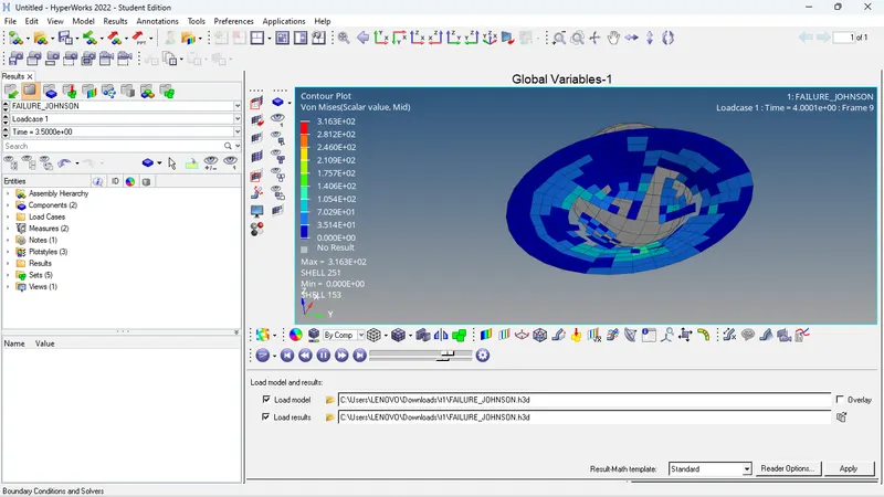
Case 1	49380	339.32s	0.8%	0	Elements are breaking and getting detached from the component	Internal energy is increasing and then becoming constant and hourglass energy is constant
Case 2	49217	327.43s	4.1%	0	Elements are breaking but not getting detached from the main component	Internal energy is increasing to its peak and hourglass is same as case 1
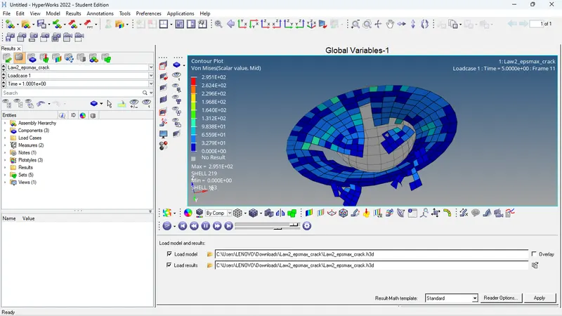
Case 3	49217	331.04s	4.1%	0	Elements are breaking and getting deatched from the main component at highest stress level.	Internal energy is increasing and Hourglass is constant
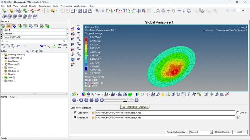
Case 4	48737	264.94s	3%	0	The elements of the main component is not breaking after removing the EPSmax value.	The increment of the internal energy is slow to the highest point creating curve graph and hour glass energy is constant.
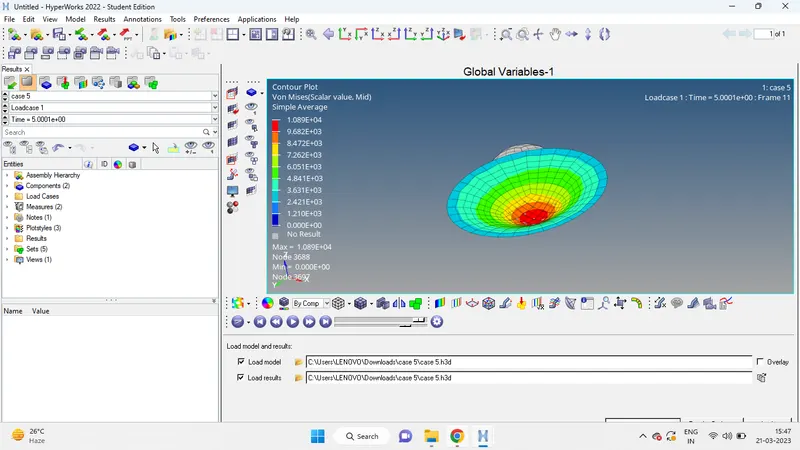
Case 5	47969	274.88s	1.3%	0	The elements of the component is not breaking even at highest strees value.	The internal energy is incresing in a curve way and hourglass energy is constant.
Case 6	48729	280.72s	0.8%	0	The elements of the component is not breaking even at highest strees value.	The internal energy is incresing in a curve way and hourglass energy is constant
Case 7	49508	293.68s	0.8%	0	Elements are breaking apart for the main compnent.	The internal energy is increasing and hourgalss energy is constant.

The images of the simulations is attached below.

Conclusion:

Observing the different simulation of the component and the Energy error and mass error by usings different Cases as mentioned.