Assignment 4-RADIOSS Material Laws Challenge
Assignment 4-RADIOSS Material Laws Challenge
Aim -
- To run the simualtion for the plate and rigid ball by using Jhonson Cook Material and Elasto Plastic Material with Brittle Failure as per the cases given in the question by using Radioss solver.
Objective -
- Run the simulation for all the 7 cases as given in the question.
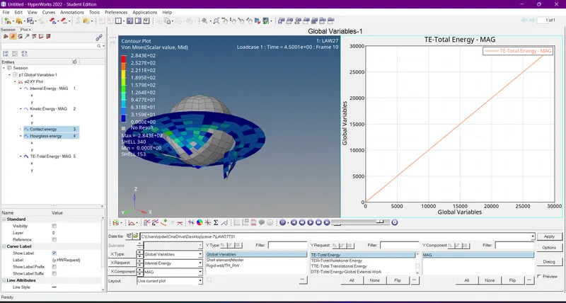
- Run the simulation by changing the material,shell properties and failure parameters.
- Run the simulation by converting Failure Jhonson Model to LAW 1.
- Tabulate the total number of cycles, Energy Error,Mass Error and Simulation Time.
- Plot the graphs for all the 7 cases.
- Compare all the 7 cases results.
Theoretical Framework -
In general, the purpose of a material is to indicate some parameters such as thickness, density, youngs modulus etc., of a component. When a material is known, So many aspects can have a solution. Like what type of analysis can be perfomed( Which includes the behavior of the material when any external forces applied on it). So, a material plays a prominent role.
In the same scenario, the materials should be specified in radioss also. Inorder to analyze it's behavior. In radioss, the materials are categorized in two ways. They are:
- Based on the form of material cards.
- Based on the material property categories.
Based on the form of material cards:-
In this method, there are so many material cards(represented in the form of laws). But Some of them are widely used in radioss, Because they were tested priorly. They are:
- Law 1 (Used to represent the elastic materials)
- Law 2 (Used to represent the Johnson-cook material).
- Law 27(Used to represent the Elasic-plastic brittle materials).
- Law 36(Used to represent the Elastic-plastic tabulated materials).
- Law 42(Used to represent the ogden materials).
- Law 70(Used to represent the foam materials).
Based on the material property categories:-
There are some majorly used materials, that are specified by the property of the materials. They are:
- Isotropic elastic materials
- Isotropic Elasto-plastic materials
- Composite & Anisotropic materials
- Viscous materials
- Hydro-dynamic materials
- Explosives
Law 1 [Isotropic Elasticity.] :
- This Law /MAT/ELAST defines an isotropic, linear elastic material using Hooke’s law. This law represents a linear relationship between stress and strain. It is available for truss, beam (type 3 only), shell and solid elements.
- Useful for elements attached to rigid body.This material law is used to model purely elastic materials.
- This law is only applicable for small deformations.
- The material stiffness is determined by only two values: the Young’s modulus (E), and Poisson’s ratio (`nu`). The shear modulus (G) can be computed using E and `nu`.
- `G=E/2(1+nu)`
| Description | Model Name | Keyword/MAT | Model Law |
| Linear Elastic | Elastic [Hooke's]. | /ELAST | 1 |
| Hyper Elastic | Tabulated Hyper Elastic. | n/a | 69 |
| Hyper Elastic | Ogden. | n/a | 82 |
Table-1
Isotropic Elasto-Plastic :
- This law represents an isotropic elasto-plastic material using the Johnson-Cook material model.
- This model expresses materialstress as a function of strain, strain rate and temperature.
- A built-in failure criterion based on the maximum plastic strain is available.
Isotropic Elastic Plastic Piecewise Linear Material [Law36] :
- This is a Isotropic elasto-plastic material.
- It's a user-defined function for the work-hardening portion of the stress-strain curve.
- It's available for brick and shell elements.
- Elastic portion of material stress-strain curve defined by Young modulus and Poisson’s ratio.
- Material plasticity curves can be given for up an arbitrary number of strain rates.
- Linear interpolation of strain-stress curve.
i) For a given strain rate.
ii) For a given plastic strain. - In order to avoid poor curve extrapolation during the strain calculation, a dummy curve defined for a high strain rate value can be added in the model—typically the highest strain rate curve is repeated.
- The curves have to be defined such as they don’t intersect themselves in the strain range being used. Otherwise the calculationmay fail.
There are 4 damage and rupture parameters :
- `εp^max`is the maximum plastic strain for element deletion for any loading (tensile , shear or compression).
- εt is the beginning of tensile damage. From this point the stress value defined in the curve is reduced by the factor
- Where ε1 is the largest principal strain `sigma=sigma(ε_m-ε_1 //ε_m-ε_t)`.
- εm is the end of the tensile damage. The stress value is null, but the element is not deleted.
- εf is the tensile failure strain value for element deletion.
Elasto-Plastic Material with Brittle Failure [Law27] :
- This law combines an isotropic elasto-plastic Johnson-Cook material model with an orthotropic brittle failure model.
- Material damage is accounted for prior to failure. Failure and damage occur only in tension. This law is applicable only for shells.
- Yield surface definition same as Johnson-Cook (Law2).
- Useful for modeling brittle failure of glass.
- Damage and rupture defined with 4 parameters for each principal direction:
`e_t` = Strain at the beginning of tensile failure.
`e_m` = Maximum tensile strain at which the stress in the element is set to a value dependent on dmax1.
`d_max` = Maximum damage factor ef = Maximum tensile strain for element deletion.
Viscous Material :
The viscous materials are classified into two types called
1) Hyper Elastic [/MAT/OGDEN or /MAT/LAW42 : Ogden, Mooney-Rivlin].
2) Tabulated Foam [/MAT/FOAM_TAB or /MAT/LAW70: Tabulated Foam].
1) Hyper Elastic [/MAT/OGDEN or /MAT/LAW42 : Ogden, Mooney-Rivlin].
- They are Visco Hyperelastic behavior (non-linear elastic).
- This law is generally used to model incompressible rubbers, polymers, foams, and elastomers.
- This material can be used with shell and solid elements.
- Generally used to model polymers and elastomers.
2) Tabulated Foam [/MAT/FOAM_TAB or /MAT/LAW70: Tabulated Foam].
- Visco-elastic behavior
- Stress – strain relationship defined by functions according to strain rate
- Unloading behavior defined by:
`***`Curves.
`***`Hysteresis Parameters.
Procedure -
Case 1
- Import the FAILURE_JOHNSON_0000.rad file and run the model as it is. Give the title name as Law2_epsmax_failure.
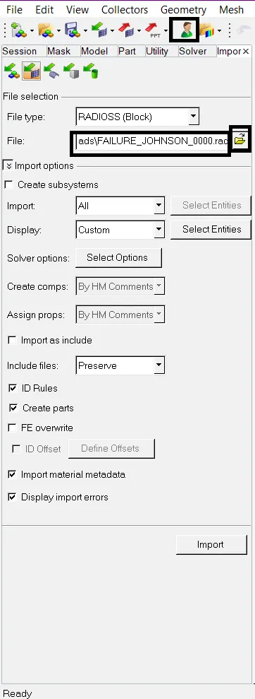
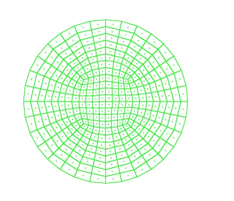
After importing the solver deck, the model appears in the graphical display
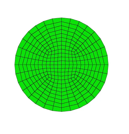
As it is seen in wireframe mode for better visualization, enable the option named "Shaded elements with mesh lines". After enabling it, the given model appears as shown in the below image.
Then in the solver browser some cards are verified, inorder to have clarity on some aspects. Among them, the first card to be checked is "Begin card". Inorder to check for the unit system. The unit system plays a prominent role for assigning all of the values. The unit system for this appears as shown in fig 5.4.
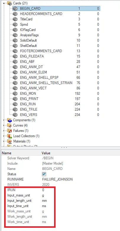
fig 5.4
The material card is the next card to be verified, in order to see the properties assigned to the material. The material card appears as shown in fig 5.5.
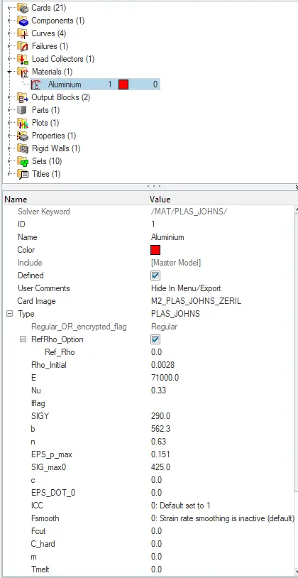
fig 5.5
The next card to be verified is the property card. In the property card, the properties assigned to the given material is seen. The property card with the assigned parameters appears as shown in fig 5.6.
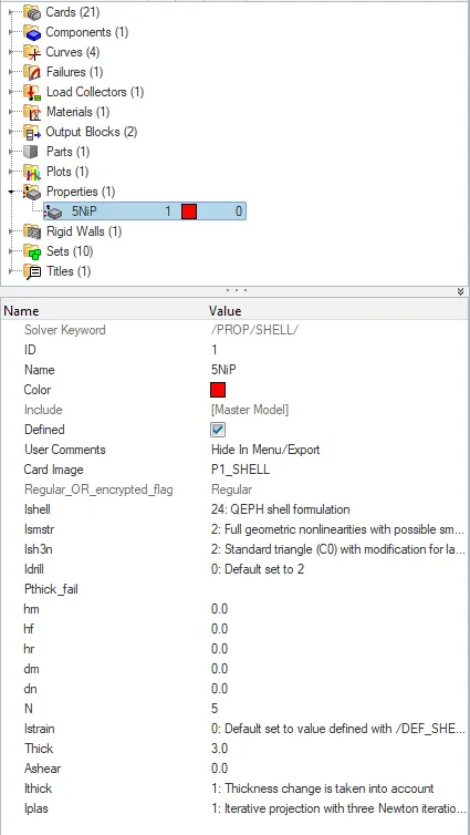
- Now run the simulation, To run the simulation, Go to Analysis Panel.
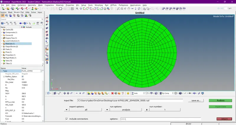
- Go to Analysis Panel >Radioss >Select the Input File > Save it in Different Folder and Rename it as Case-1 > Run.
- Check the Include Connectors, If there are any connectors in the model, The connectors will also be taken into account.
- Type -NT 4 in the options tab, This will make the simulation faster.
- Where NT indicates No of threads,4 indicates assigning the task to 4 cores in the system.
-
Here save the input file in a different folder, and rename it as case-1 which
- Now run the solver by hitting on radios.
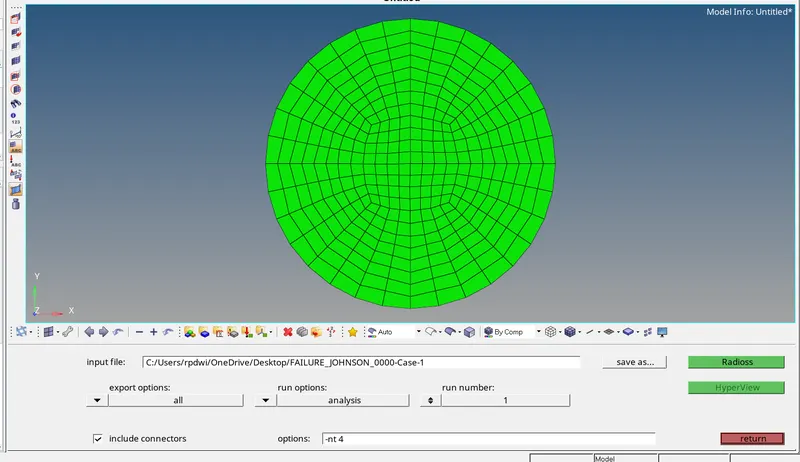
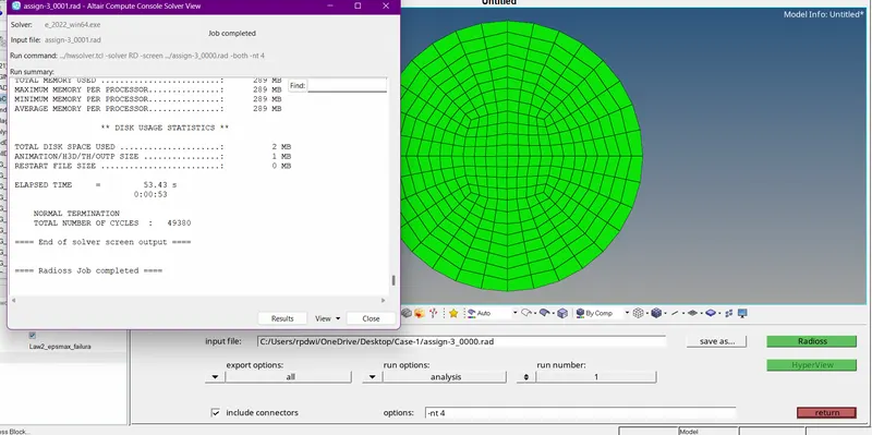
After completing the simulation,the radioss will pop up a solver window stating Radioss Job Completed which indicates the simulation has been completed
After running the simulation,The animation files will be generated where we specified a location to store the files
- Now go and open the 00001.out file with notepad.
- The obtained values for Energy Error,Mass Error,Internal Energy Error,Kinetic Energy Error and Contact Energy Error
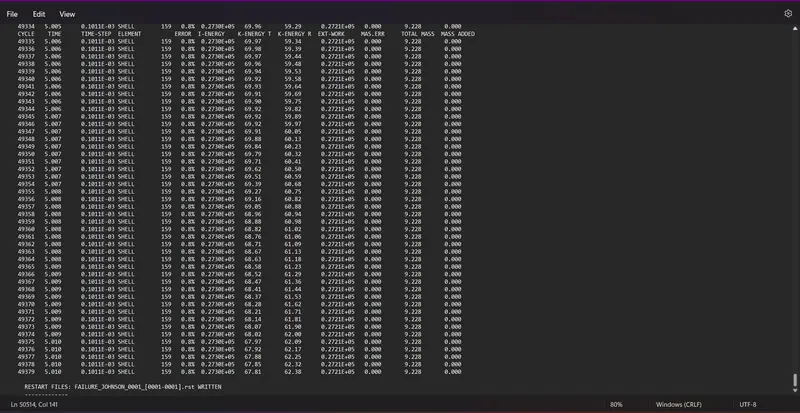
- The values obtained for this cycle are
Energy Error-0.8%
Internal Energy-0.2730E+05
Kinetic Energy-67.81
External Work-0.2721E+05
Elapsed Time-95.36s
Mass Error-0
Total No of Cycles-49380
- Next the 00001.rad file is opened to see the Tstop and Tfrequency value which is shown in below figure 16.
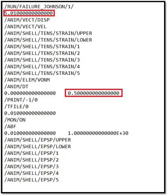
Postprocessing of Case-1
1) Review the Simulation using -HyperView.
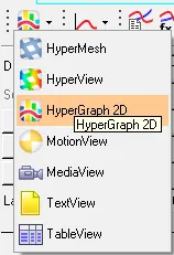
2) Plot the graphs using -Hypergraph 2D.
1) Review the Simulation using HyperView :
-
- After analysis go for the hyper view to run the animation file.

- Apply after importing the file and the mesh model is ready for the animation as below shown.
- After importing the .h3d file into the GUI, Enable the contour. The contour tool creates contour plots of a model and graphically visualizes the analysis results.
- To enable contour, Go to Results Toolbar → Contour.
- Import the animation file .h3d into the hyperview.
- After loading the model into hyperview,It will be represented as shown in below.
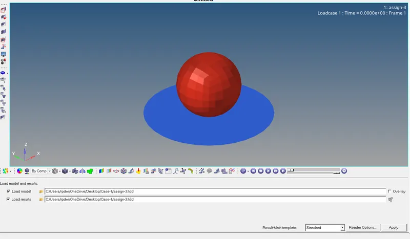
- After applying ,Run the Simulation,The Simulation animation is shown in below Figure 24.
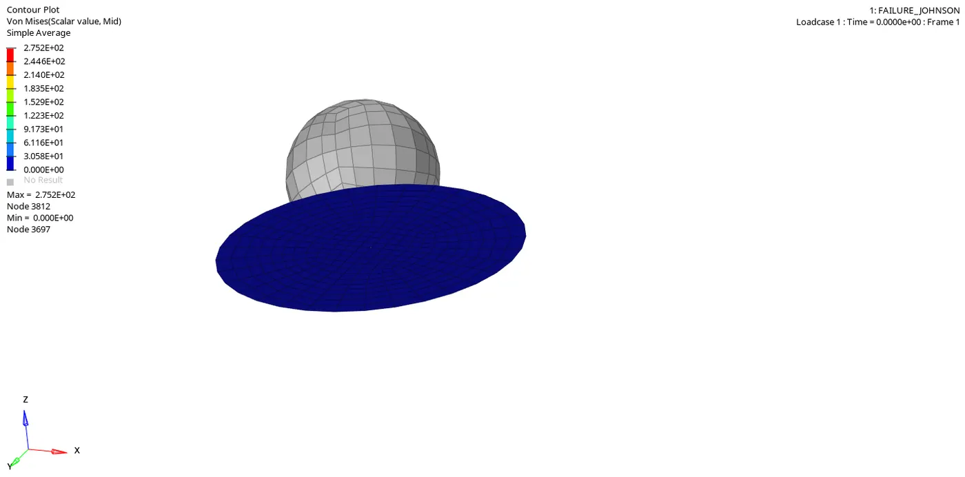
| Figure 24-Case 1-HyperView Simulation Animation. |
- On the basis of the animation, plot the graph for the various energy for the given component.
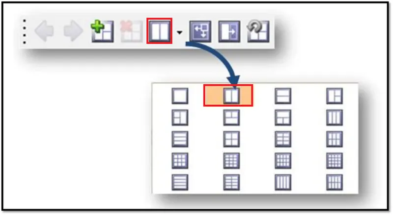
The pages can be split into 2 so that perform the other operations in to account. Use the expand and reduce the window.
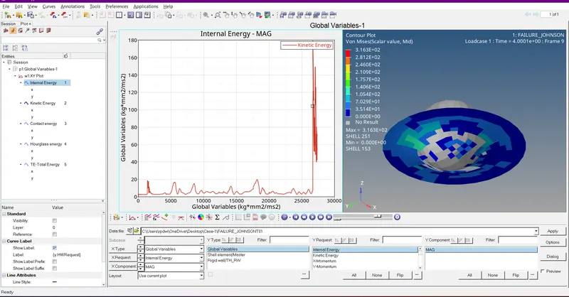
Kinetic Energy :
- The kinetic energy decreases, why because the velocity decreases (The rail component starts to deform, and after complete deformation, it will be in rest) when the component comes to a rest, So velocity becomes zero and the kinetic energy decreases.
- The imposed velocity is for the rigid ball, Why because we are imposing the rigid ball to hit on the rupture plate, So that's the reason, why imposed velocity is given?
- The formula for Kinetic Energy=1÷2mv^2
- Here the initial velocity is zero, So the curve starts from the origin.
- After its increasing, because the rigid ball is hitting the rupture plate and again it slightly decreases due to element breakage After the elements are deleted, there will be no contact, So it's decreasing.
Why Kinetic Energy Curve is Zig-Zag ?
- Cause Noise and Vibrations will be produced when the rigid ball hits the rupture plate, so the kinetic energy curve is in Zig-Zag form.
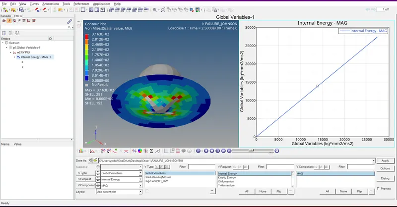
Internal Energy:-
- Usually, the internal energy starts from the origin, And it increases because of the increase in displacement.
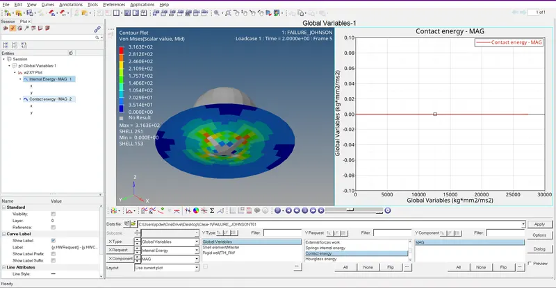
Contact Energy:-
Why contact energy is constant?
- Because the rigid ball is a rigid body and the rupture plate is a deformable body, So the contact energy is constant.
- If deformable bodies get in contact, then only the contact energy increases.
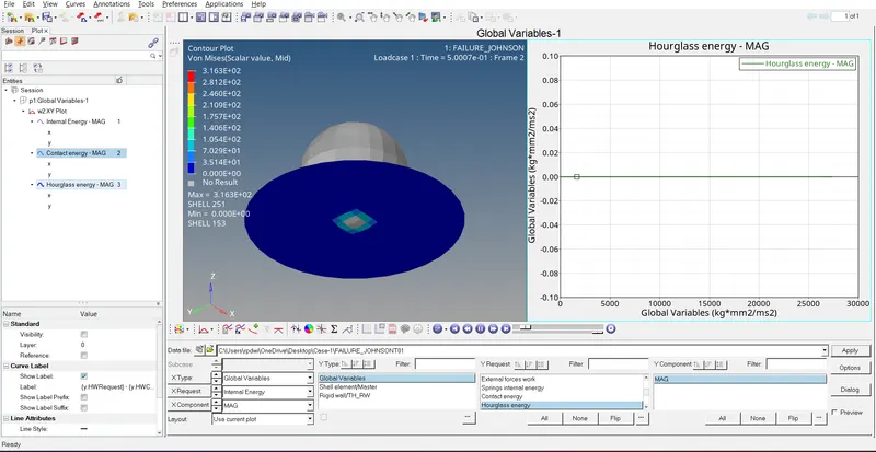
Hourglass Energy:-
- Here the hourglass energy is constant, Because the recommended parameter Ishell=24 has been assigned to the property card, So the hourglass energy is constant
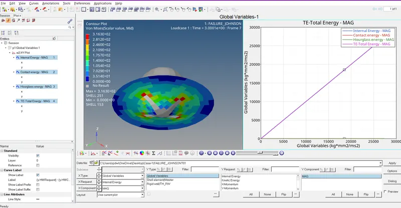
Total Energy:
- Total Energy is the sum of Kinetic Energy+Contact Energy+Hourglass Energy + Internal Energy.
- Total Energy is the combination of all energies.
- So it goes on increasing, Internal energy curve is similar to the total energy.
Case 2:-Change the Values in Jhonson Failure Card
- Import the case 1 rad file, named “Law2_epsmax_failure” and perform the simulation with failure plastic strain (EPS_p_max) and fail_Johson card enabled.
- Changes to be made in /FAIL/JOHNSON card:
- ifail_sh= 1
- Dadv= 1
- Ixfem= 1
- Use the recommended values for the property card.
- Give the title name as Law2_epsmax_crack.
In this case import the case-1 file gives the title name as Law2_epsmax_crack and the material is the same before going to the simulation part change the property card value as recommended in case-2. 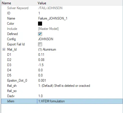
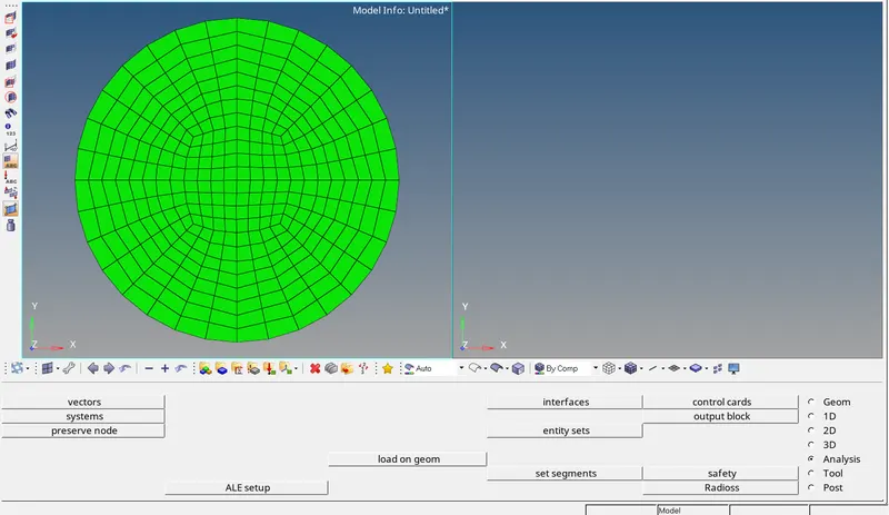
Now run the simulation using radioss,After running the simulation,The animation and TH files will be obtained in a required location.
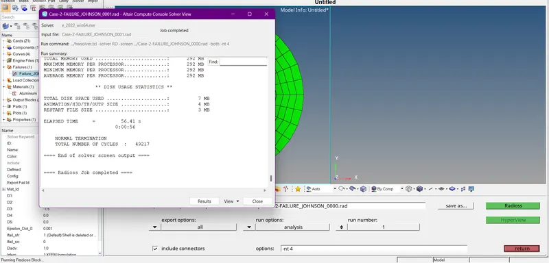
After completing the simulation,the radioss will pop up a solver window stating Radioss Job Completed which indicates the simulation has been completed
- Now go and open the 00001.out file with notepad.
- The obtained values for Energy Error,Mass Error,Internal Energy Error,Kinetic Energy Error and Contact Energy Error has been shown in below.
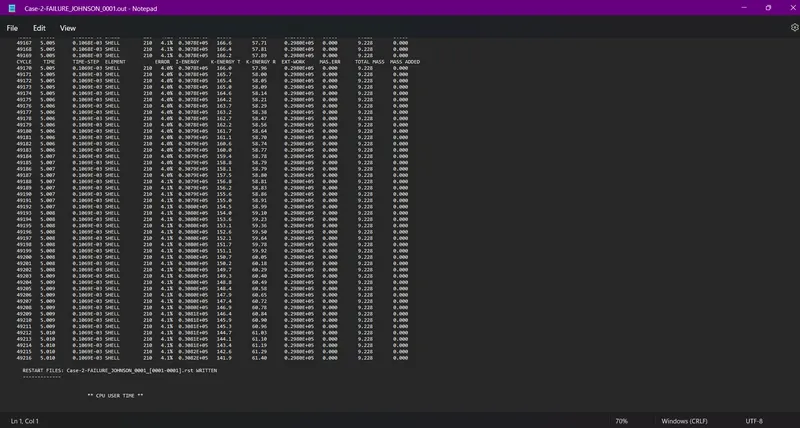
The obtained last cycle values are:
energy error = 0.2%
Internal energy = 0.2708E+05 KJ
Kinetic energy = 113 .6 KJ
External work = 0.2721E+05 KJ
Mass error = 0
elapsed time = 114.38 s
Total number of cycles = 49217
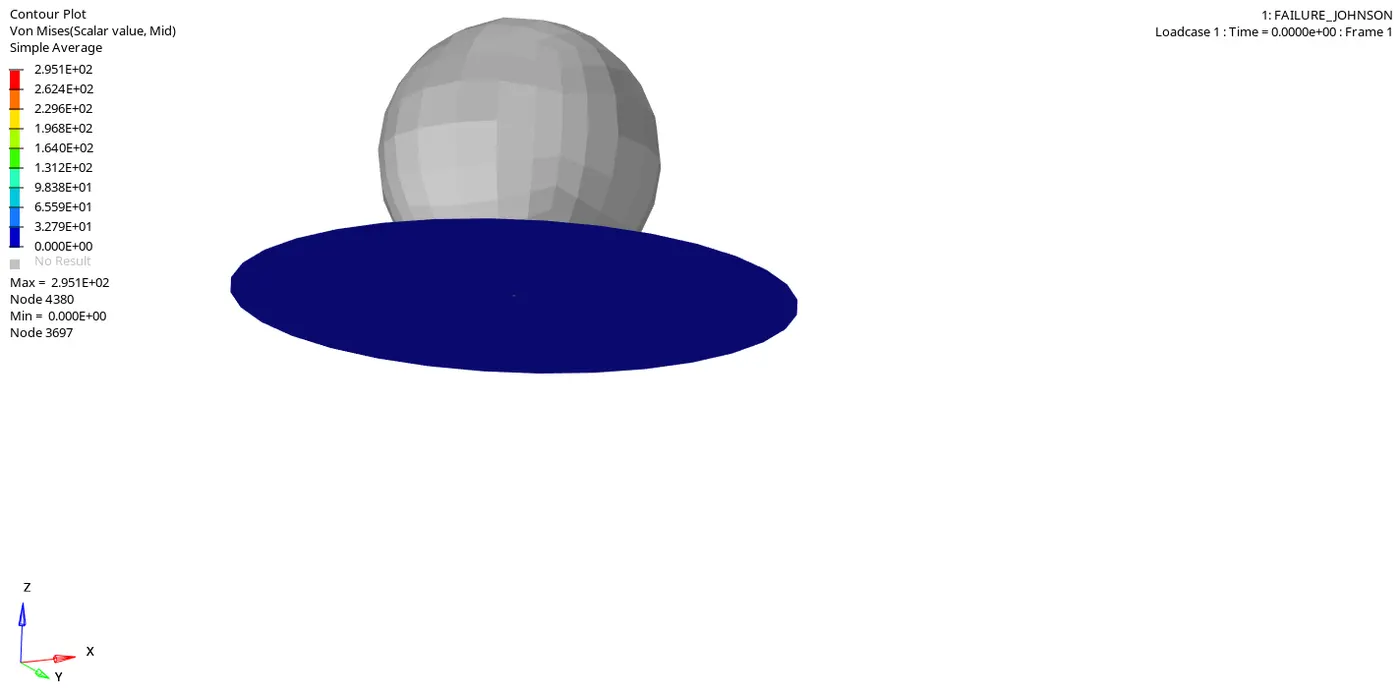
The obtained h3d file is imported in the hyperview, in order to simulate. The obtained simulation appears as shown in the below animation.
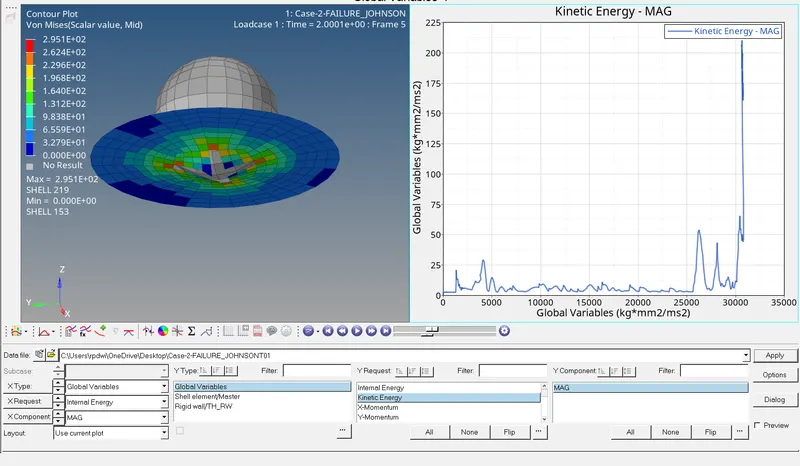
Kinetic Energy :
Here the kinetic energy starts from origin and goes on increasing due to deformation of elements,Its increasing after 4ms because the deformation of elements are controlled by jhonson cook material parametrs.And its suddenly decreasing because the elements getting deleted after crack and there will no contact,so its slightly decreasing.
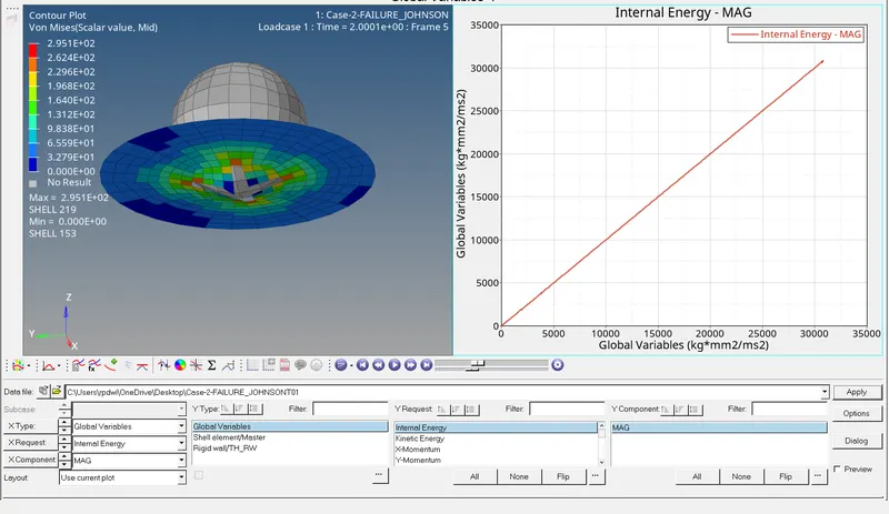
Internal Energy :
Here the curve is starting from origin because there is no contact and its goes on increasing due to the breakage of elements.
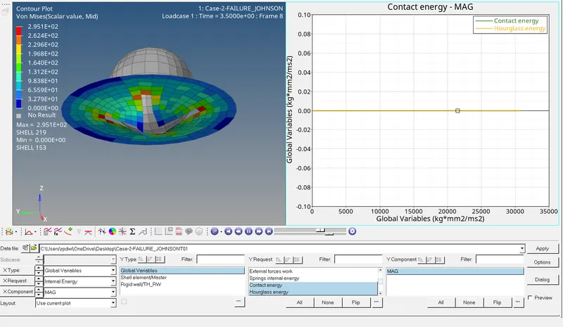
Contact Energy-
- Because the rigid ball is rigid body and the rupture plate is deformable body,So the contact energy is constant.
- If deformable bodies get in contact,then only the contact energy increases.
Hourglass Energy-
Here hourglass energy is constant due to recommended parameters have been assigned.Here Ishell=24 QEPH is used,Due to this there is no houglass effect.
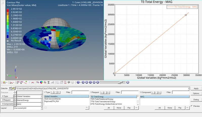
Total Energy :
- Total Energy is sum of Kinetic Energy+Contact Energy+Hourglass Energy + Internal Energy.
- Total Energy is the combination of all energies.
- So its goes on increasing,Internal energy curve is similar to the total energy.
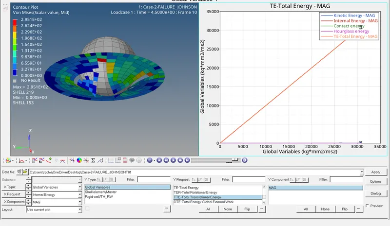
Case 3-Delete the Failure Jhonson Card
- Here the failure card is deleted to see any changes happening the result.
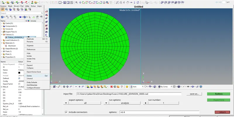
Now run the simulation using radioss, After running the simulation, The animation and Th files will be obtained in the required location.
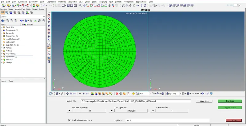
After completing the simulation,the radioss will pop up a solver window stating Radioss Job Completed which indicates the simulation has been completed
- Now go and open the 00001.out file with notepad.
- The obtained values for Energy Error,Mass Error,Internal Energy Error,Kinetic Energy Error and Contact Energy Error has been shown in below
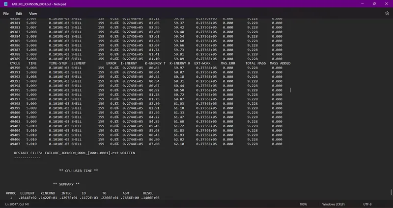
The obtained maximum values are:
energy error = 0.8%
Internal energy = 0.2744E+05 KJ
Kinetic energy = 87.08 KJ
External work = 0.2736E+05 KJ
Mass error = 0
elapsed time = 112.73 s
Total number of cycles = 49408
1) Review the Simulation using -HyperView.
- After completion of running the simulation,Switch to the hyperview.
- Open the appropriate .h3d file to review the simulation.
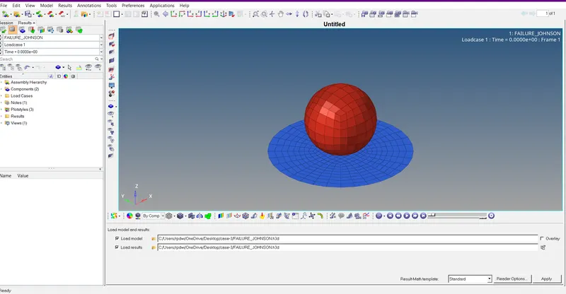
- The .h3d file is loaded
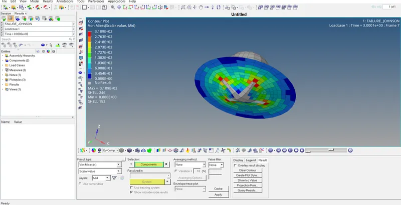
- Here the shell elements are getting deleted,when it reaches the maximum plastic strain eps max value which is shown in below animation.
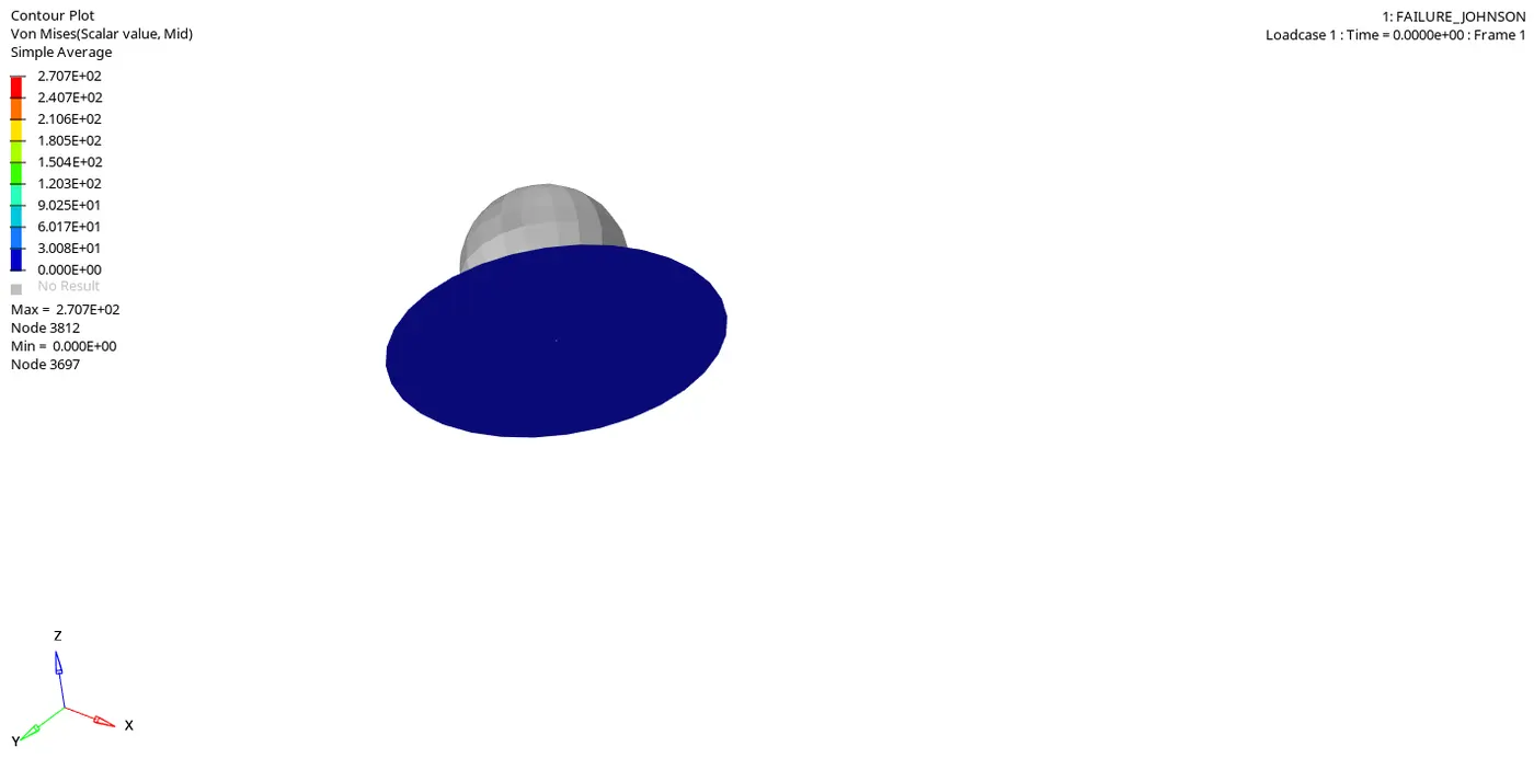
From the above animation, noticed thing is that, the elements break because, the circular plate is assigned with elasto-plastic material.
2) Plot the graphs using-Hypergraph 2D.
- Now switch to the Hypergraph 2D and plot the graphs.
Internal Energy:-
Then the internal energy is plotted, it appears as shown in below image. This will be some what similar to the previous cases. 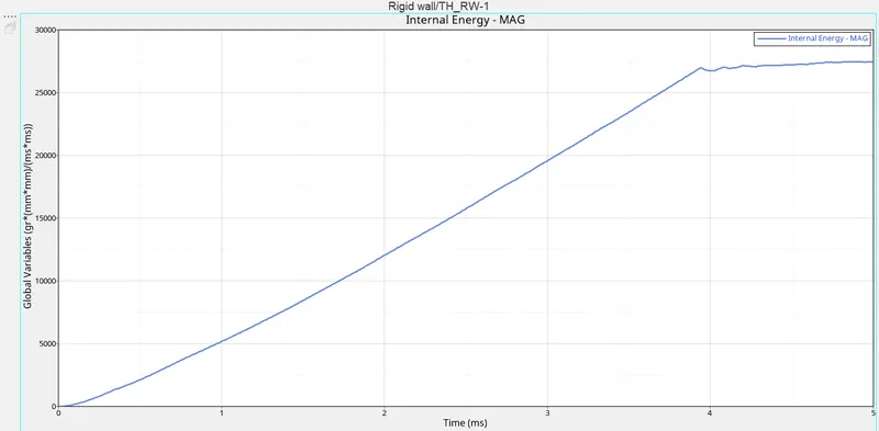
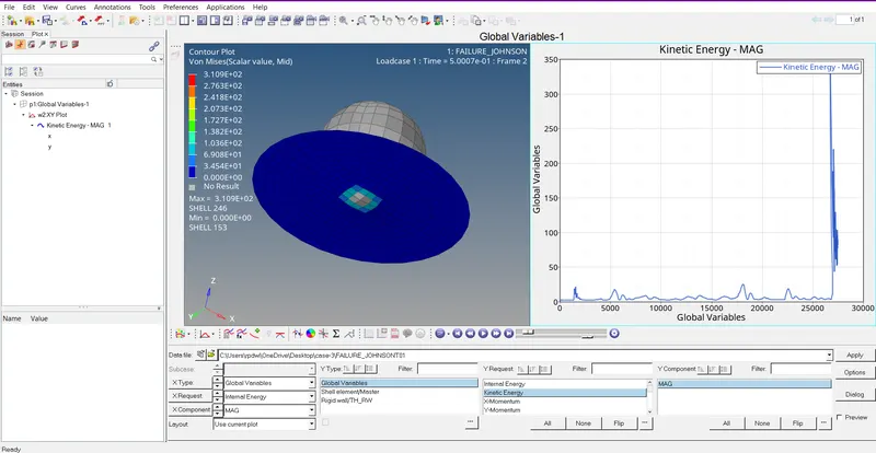
Kinetic Energy:-
The kinetic energy obtained here is somewhat less when compared to the previous case,The obtained kinetic energy graph.
Contact Energy-
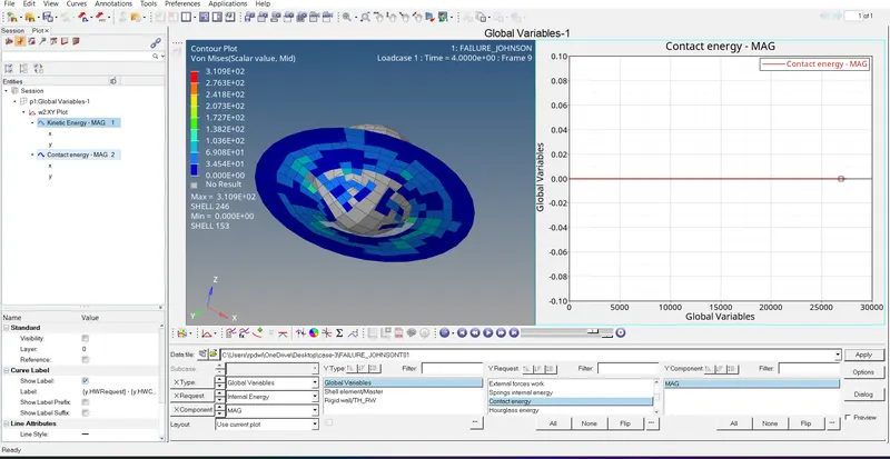
Then the Contact energy is plotted, it appears as shown in below image. This will be some what similar to the previous cases.
Hourglass energy:-
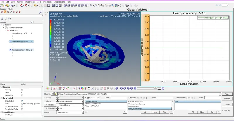
- Here hourglass energy is constant due to recommended parameters have been assigned.Here Ishell=24 QEPH is used,Due to this there is no houglass effect.
- Simillarly as same as for case-3.
- Because the rigid ball is rigid body and the rupture plate is deformable body,So the contact energy is constant.
- If deformable bodies get in contact,then only the contact energy increases.
- The obtained hourglass and contact energy graph
Total Energy:-
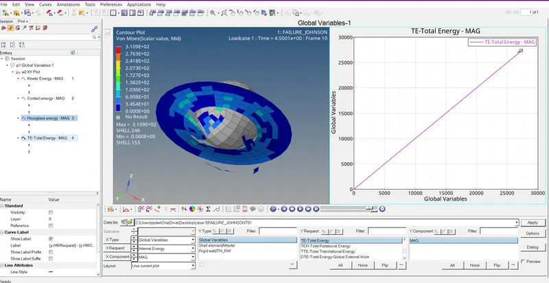
- The total energy increases with increase in internal energy and kinetic energy,Cause the total energy is combination of all energies.
- The obtained total energy graph
Case 4 - Delete the EPS_P_Max Value from the Material Card :
In this case for the same material card, the plastic strain(eps_max) value which is 0.151 as shown in fig 5.38, is removed(eps_max).
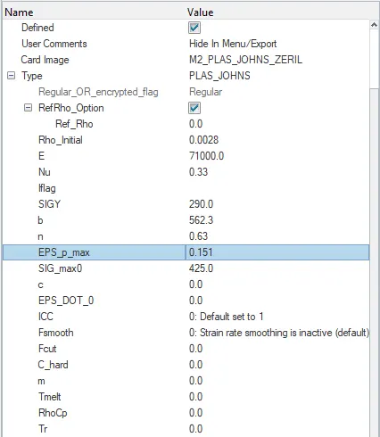
fig 5.38
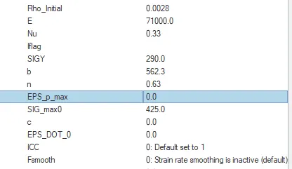
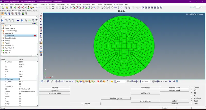
After removing the value for plasic strain, the material card appears as shown in fig 5.39.
Now run the simulation using radioss,After running the simulation,The animation and TH files will be obtained in a required location,
- Now go and open the 00001.out file with notepad.
- The obtained values for Energy Error,Mass Error,Internal Energy Error,Kinetic Energy Error and Contact Energy Error
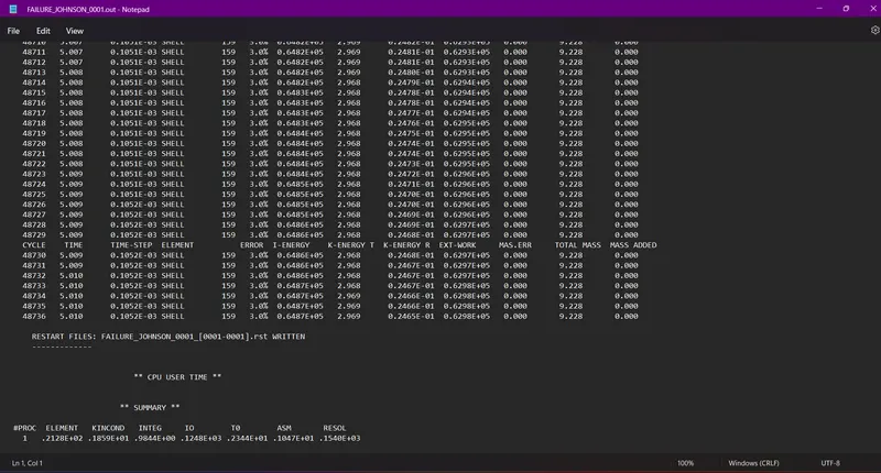
The obtained last cycle values are:
energy error = 1.1%
Internal energy = 0.3879E+05 KJ
Kinetic energy = 3.931 KJ
External work = 0.3838E+05 KJ
Mass error = 0
elapsed time = 141.41 s
Total number of cycles = 49304
1) Review the Simulation using -HyperView.
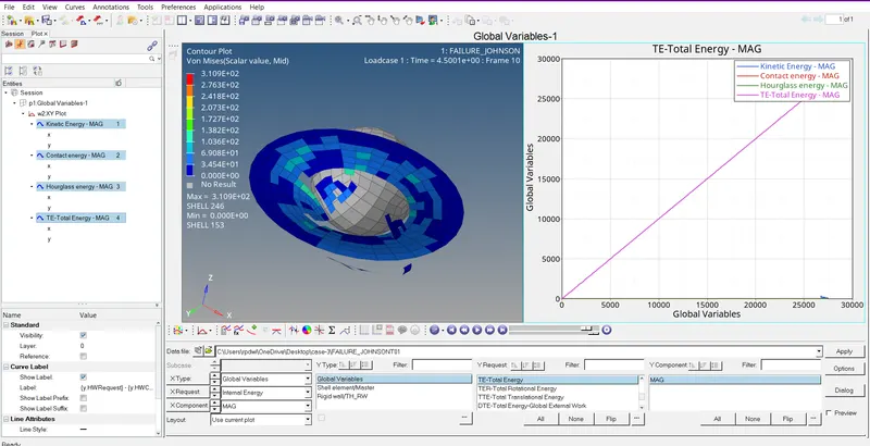
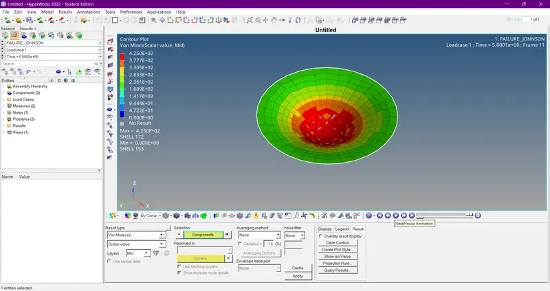
Then the obtained h3d file is imported in the another window, In order to view the simulation. The obtained simulation in terms of von-mises is shown in below animation. As the eps_max value (plastic strain) is zero, the elements will not break.
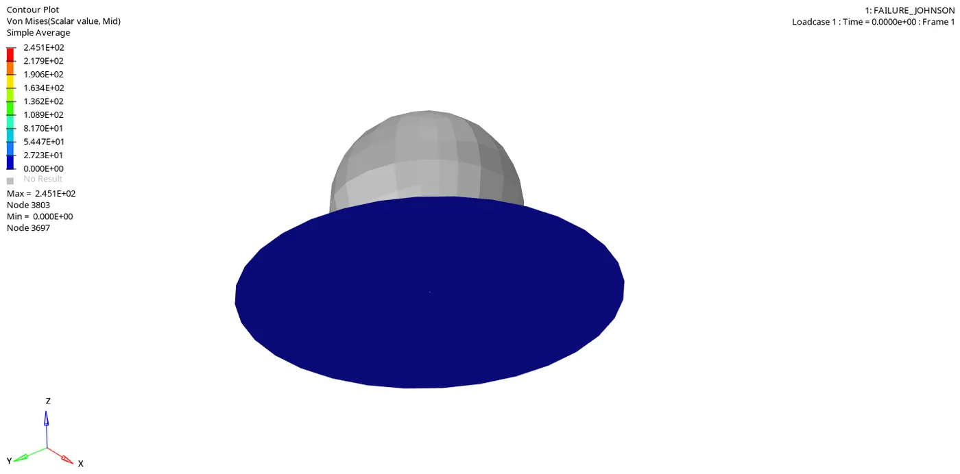
The elements are not getting deleted.
2) Plot the graphs using-Hypergraph 2D.
- Now switch to the Hypergraph 2D and plot the graphs.
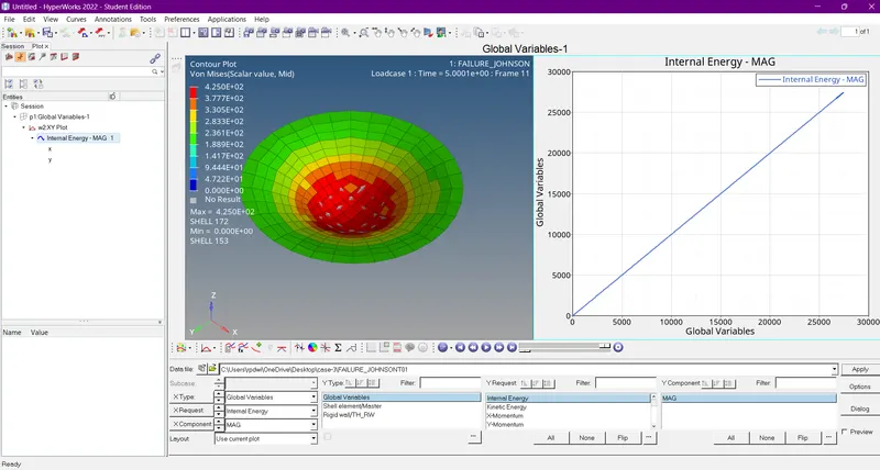
- The internal energy graph is plotted which is shown below in Figure 64,her internal energy is somewhat similar to the previous case.
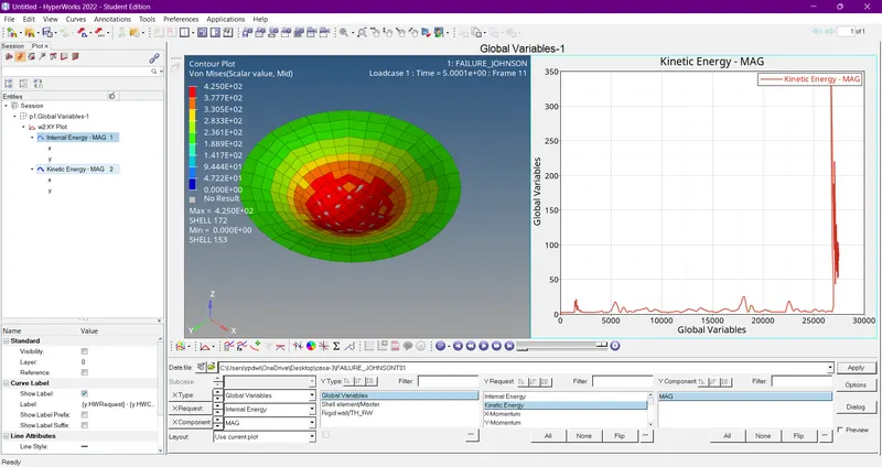
- The kinetic energy is plotted, which is shown in below Figure 65.The kinetic energy is also somewhat similar to the previous case.
- Kinetic Energy produced here is little bit less cause deformation of elements is happening slowly.
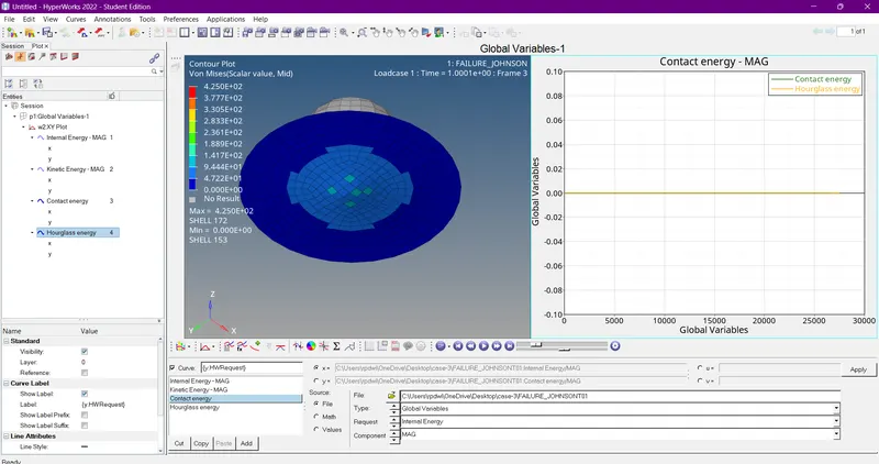
- Here hourglass energy is constant due to recommended parameters have been assigned.Here Ishell=24 QEPH is used,Due to this there is no houglass effect.
- Simillarly as same as for case-4.
- Because the rigid ball is rigid body and the rupture plate is deformable body,So the contact energy is constant.
- If deformable bodies get in contact,then only the contact energy increases.
- The obtained hourglass and contact energy graph is shown in above
Total Energy :
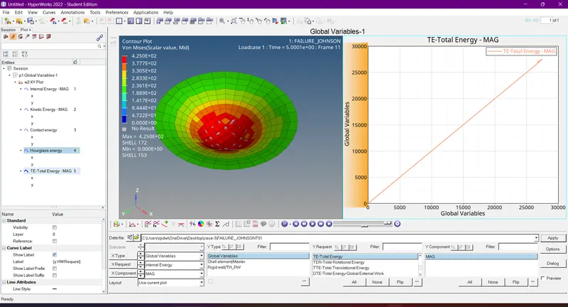
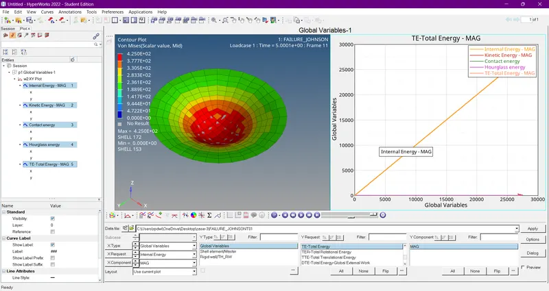
- The total energy is almost similar to the internal energy.
- The total energy graph is plotted which is shown in below image.
Case 5 - Change the Material Card to LAW1 :
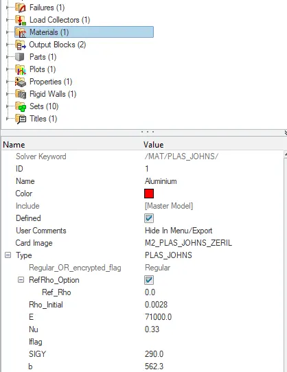
- Import the case 4 rad file and perform the simulation by changing the material card to Law 1. Keep the same value for rho, E, and nu values.
- Now go and open the 00001.out file with notepad.
- The obtained values for Energy Error,Mass Error,Internal Energy Error,Kinetic Energy Error and Contact Energy Error has been shown in below image
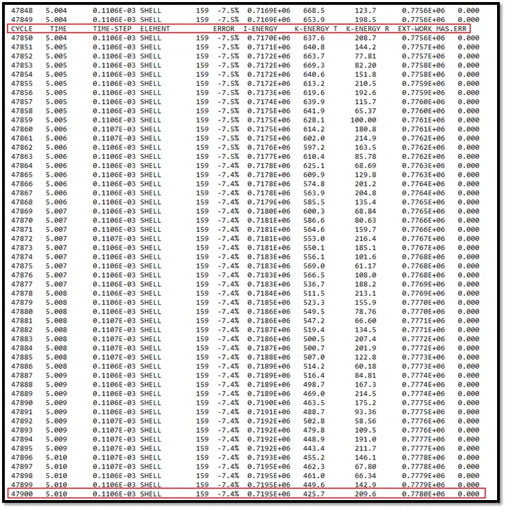
Obtained values for Energy Error,Mass Error,Internal Energy Error,Kinetic Energy Error and Contact Energy Error
- The values obtained for this cycle are
The obtained values for last cycle are:
energy error = 1.3%
Internal energy = 0.8632E+06 KJ
Kinetic energy = 1677 KJ
External work = 0.8568E+06 KJ
Mass error = 0
elapsed time = 107.94 s
Total number of cycles = 47969
1) Review the Simulation using -HyperView.
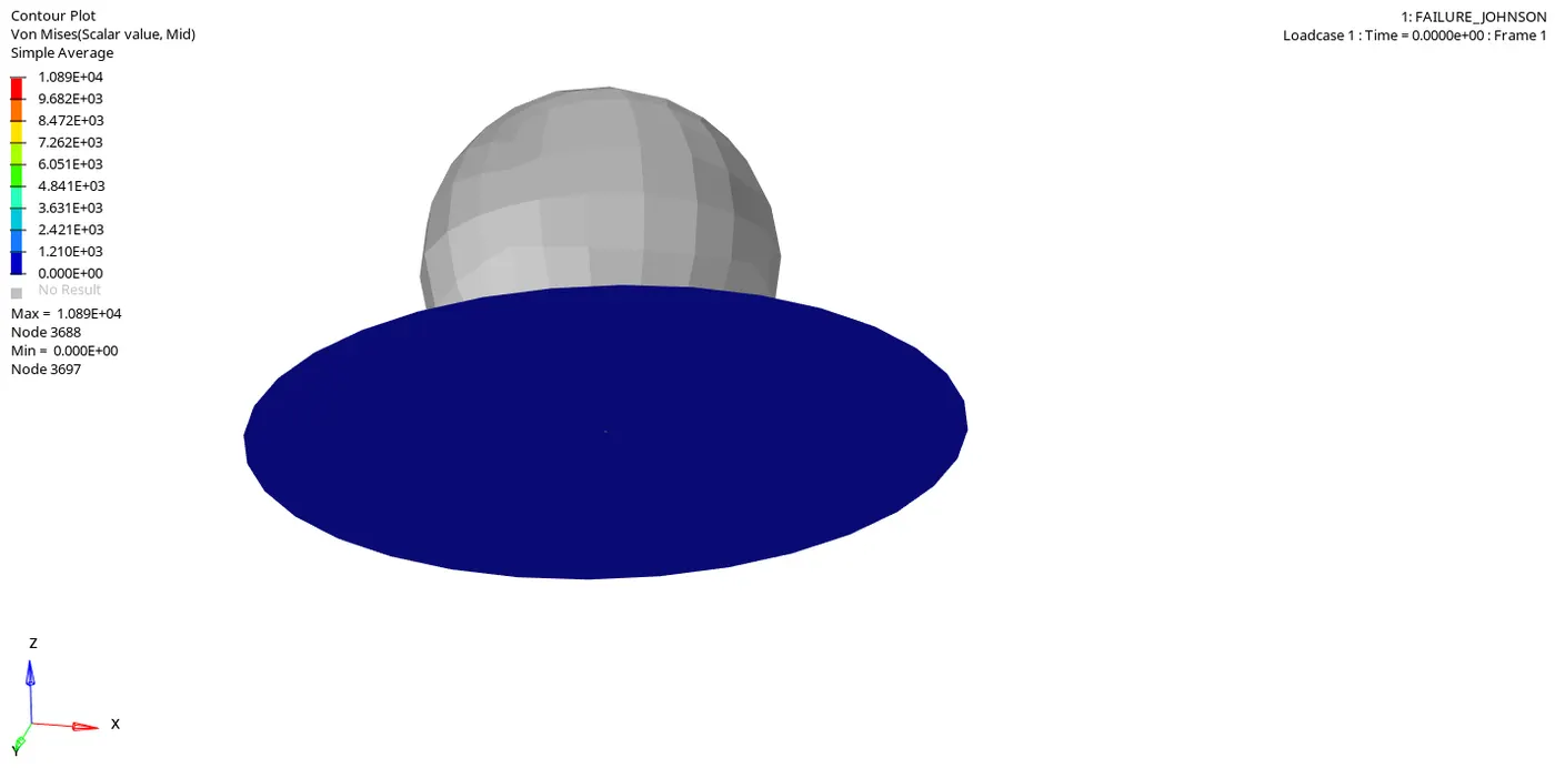
Then the obtained h3d file is imported in the another window, In order to view the simulation. The obtained simulation in terms of von-mises is shown in below animation. The elements will not even split during the collision. Because, the law 1 is assigned to the circular plate. So, it possess the elasticity (i.e., abitlity to regain its original size & shape).
2) Plot the graphs using-Hypergraph 2D.
Then the graphs are plotted to view the results. The total resultant force of the rigid wall force increases gradually till the end. Because, there is no plastic behavior seen in this case. The obtained rigid wall force graph appears as shown in the below graph image.
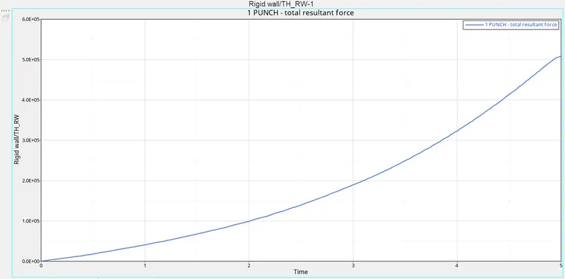
fig 5.51
Then the internal energy graph is obtained, as shown in the below graph image. Internal energy also increases gradually. But the graph will be some what dissimilar to that of the previous cases.
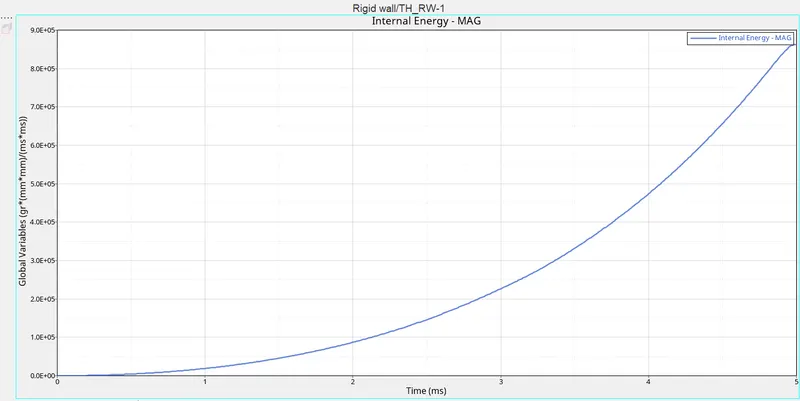
fig 5.52
Then the kinetic energy is plotted, appears as shown in below graph image. Initially, the kinetic energy is constant. And it varies when the rigid sphere hits the circular plate & it reaches to the peak value when the elements absorbs the more energy at the end of collision.
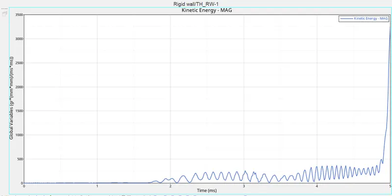
fig 5.53
As the property assigned is with the recommended parameters such as the QEPH element with Ishell:24 is used, there will be no hourglass energy(Because, it will have integrated hourglass enenrgy). So, the hourglass energy is constant as shown inbelow graph image.
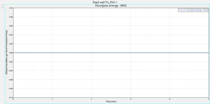
fig 5.54
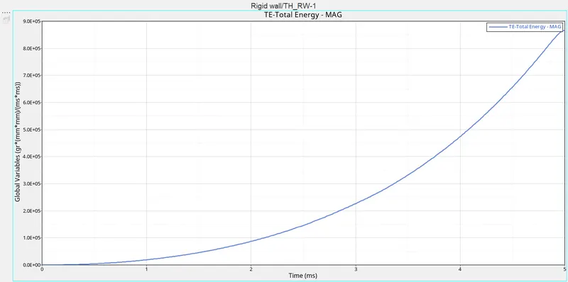
Total energy increases with the increase in internal energy & kinetic energy. The obtained total energy appears as shown in below graph image. And it keeps on increasing just similar to the internal energy. And the graphvaries when compared to the other cases.
Case 6-Change the Material Card to LAW27 :
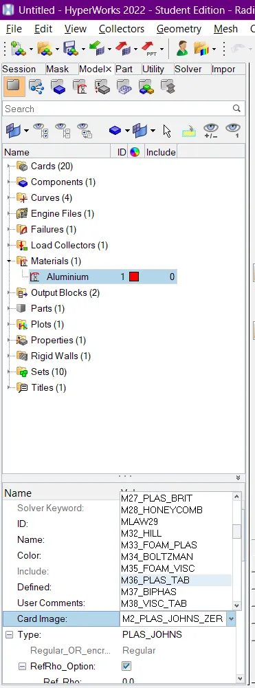
- Here change the material card to LAW27 and change the shell properties to the recommended shell peroperties.
- It is an isotropic elastoplastic jhonson cook material model with an orthographic brittle failure model.
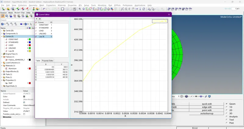
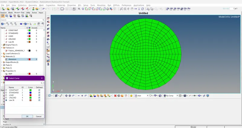
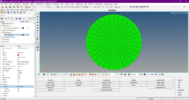
While defining the material card as law 36, a function should be represented to define the curves. Initially, there will be some curves are defined. But a new curve is defined, the values are given by the user as shwon in image A curve will be generated based on the given values.
Higher the curve> Higher the strain rate> But earlier the failure takes place.
The process of creating the curve is: create> curve> New> assign a name> proceed> shows the curve with values & graph.
- Now go and open the 00001.out file with notepad.
- The obtained values for Energy Error,Mass Error,Internal Energy Error,Kinetic Energy Error and Contact Energy Error has been shown in below image
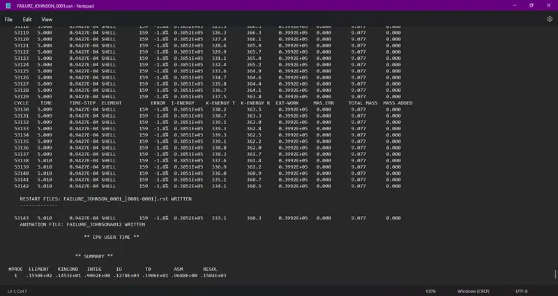
The obtained values for last cycle are:
energy error = 1.4%
Internal energy = 0.4326E+05 KJ
Kinetic energy = 159.4 KJ
External work = 0.4426E+06 KJ
Mass error = 0
elapsed time = 121.3s
Total number of cycles = 53202
1) Review the Simulation using -HyperView.
Then the obtained h3d file is imported in the another window, In order to view the simulation. The obtained simulation in terms of von-mises is shown in below animation.
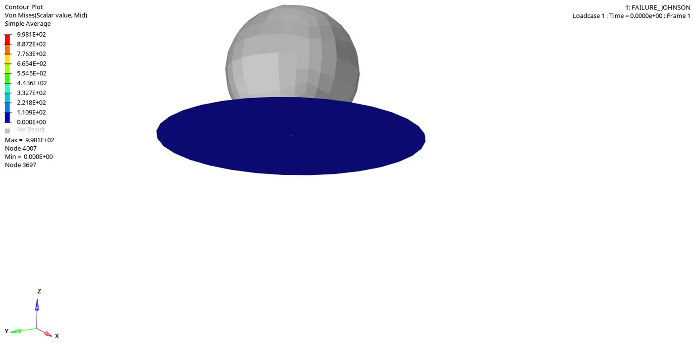
In this case also the elements will break. Beacuse, the material card assigned possess both elastic & plastic material.
2) Plot the graphs using-Hypergraph 2D.
The rigid wall forces obtained are shown in the form of graph as shown inthe below image.
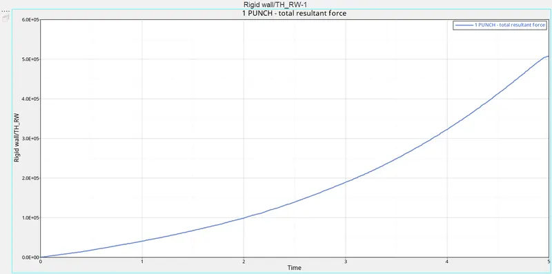
fig 5.60
The obtained internal energy in the form of graph appears as shown in the below image. The internal energy increases gradually same as in previous case.
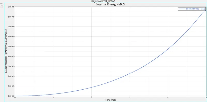
fig 5.61
Then the obtained kinetic energy graph is plotted, shown inthe below image.
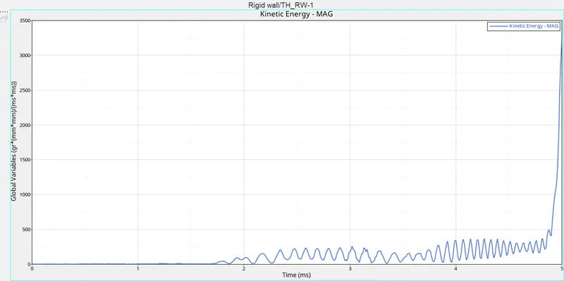
fig 5.62
As the property assigned is with the recommended parameters such as the QEPH element with Ishell:24 is used, there will be no hourglass energy(Because, it will have integrated hourglass enenrgy). So, the hourglass energy is constant as shown in the below image.
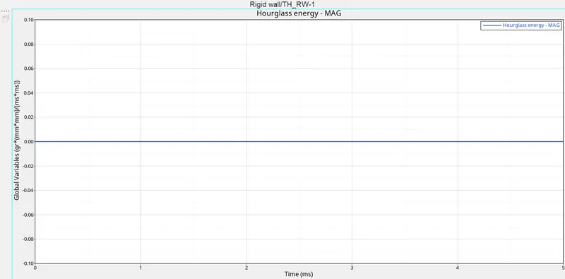
Total energy increases with the increase in internal energy & kinetic energy. The obtained total energy appears as shown in the below image. And it keeps on increasing just similar to the internal energy.
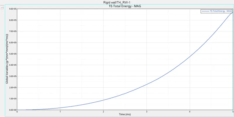
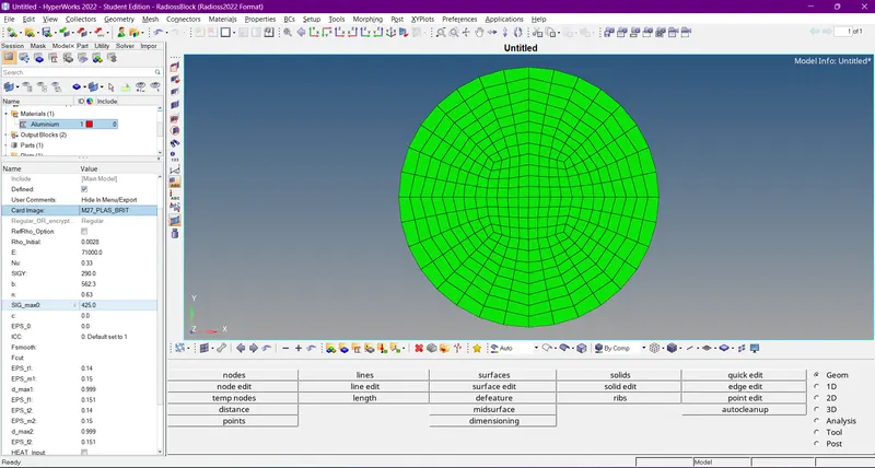
Case 7- Change the Material Card to LAW36 :
- Here change the material card to LAW36.
- A shell parameters are changed to the recommended parameters.
- It's a elasto plastic piecewise linear material
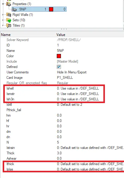
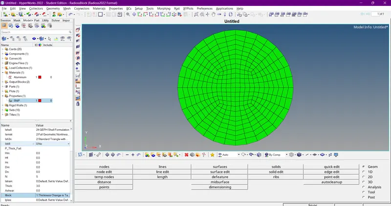
fig 5.65
After changing the parameters in the property card, it appears as shown in fig 5.66.
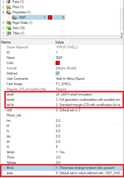
fig 5.66
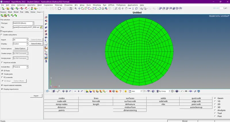
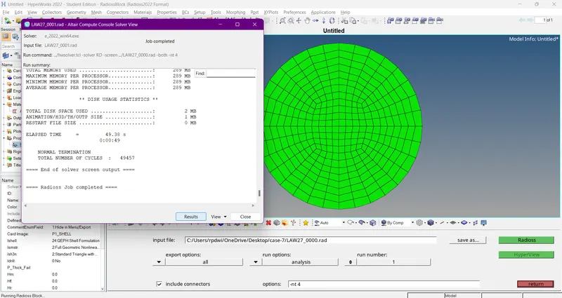
- Now go and open the 00001.out file with notepad.
- The obtained values for Energy Error,Mass Error,Internal Energy Error,Kinetic Energy Error and Contact Energy Error has been shown in below image.
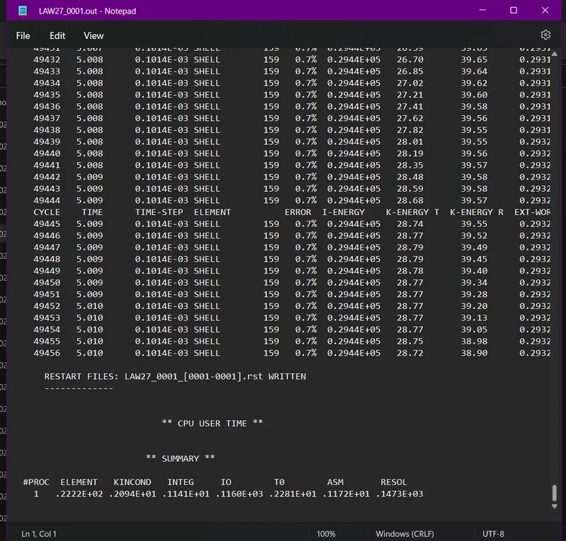
The obtained values for last cycle are:
energy error = 0.7%
Internal energy = 0.2936E+05 KJ
Kinetic energy = 53.59 KJ
External work = 0.2927E+05 KJ
Mass error = 0
elapsed time = 112.75 s
Total number of cycles = 49468
1) Review the Simulation using -HyperView.
Then the obtained h3d file is imported in the another window, In order to view the simulation. The obtained simulation in terms of von-mises is shown in below animation. Here the elements will break due to its brittle property.
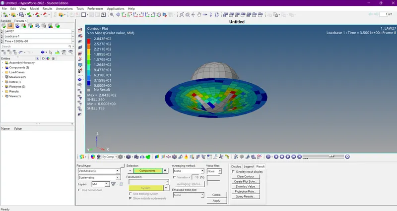
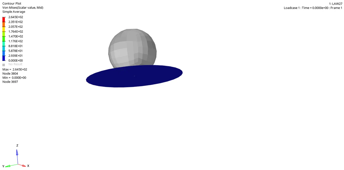
2) Plot the graphs using-Hypergraph 2D.
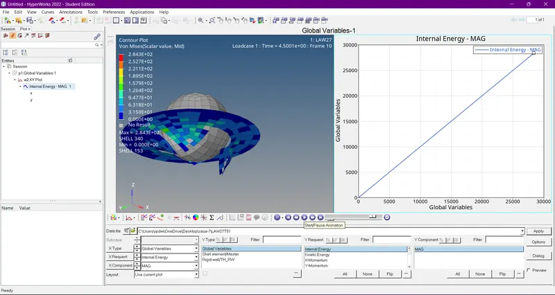
Internal Energy :
- The internal increases as same as in previous case.
- The obtained graph for internal energy is shown in below image
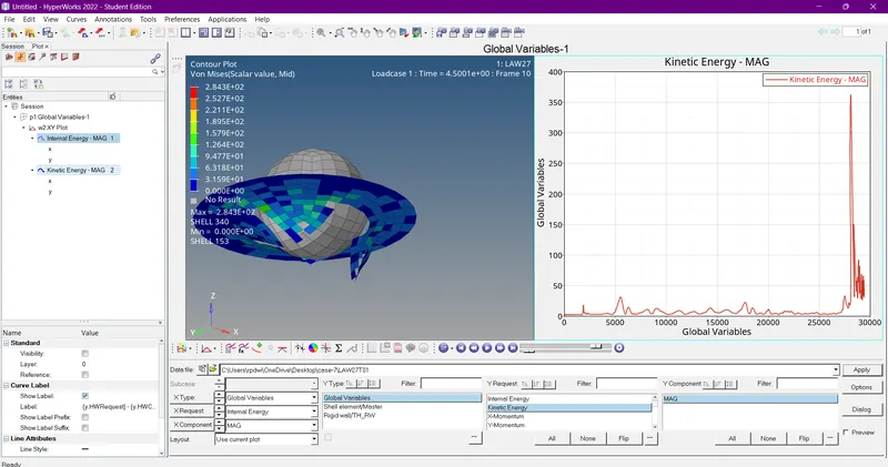
Kinetic Energy :
- The kinetic energy is somewhat similar to the case-5.
- The obtained kinetic energy graph is shown in below image
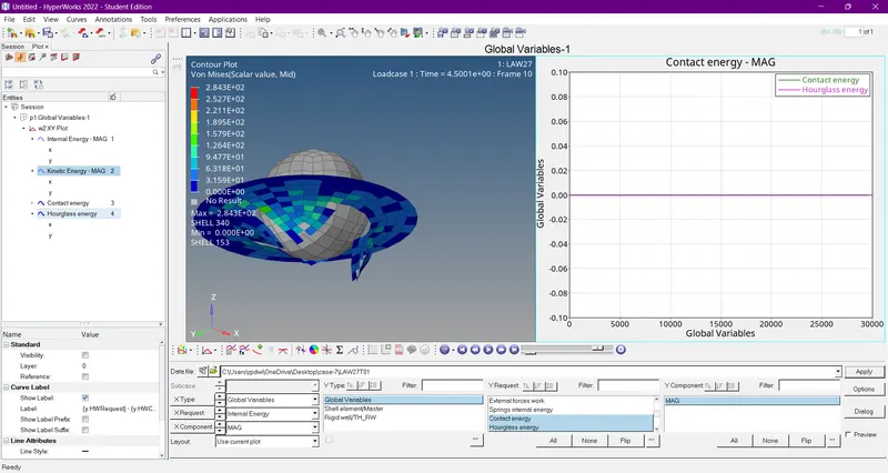
Hourglass and Contact Energy :
- Here hourglass energy is constant due to recommended parameters have been assigned.Here Ishell=24 QEPH is used,Due to this there is no houglass effect.
- Simillarly as same as for case-7.
- Because the rigid ball is rigid body and the rupture plate is deformable body,So the contact energy is constant.
- If deformable bodies get in contact,then only the contact energy increases.
- The obtained hourglass and contact energy graph is shown in below
Total Energy :
- The total energy increases with increase in internal energy and kinetic energy.
- The obtained graoh for total energy is shown in below
Comparison of all the 7 Cases :
| Cases | Energy Error | Internal Energy | Kinetic Energy | External Work | Mass Error | Elapsed Time | Total Number of Cycles | Material Used | Changes in Material Parameters | Element Failure Behaviour |
| Case-1 | 0.8% | 0.2730E+05 | 67.81 | 0.2721E+05 | 0 | 95.36s | 49380 | Jhoonson-Cook [LAW2] | Used Default Shell Parameters and Runned the Simulation. | Elements Deleted. |
| Case-2 | 4.1% | 0.3082E+05 |
141.9
|
0.2980E+05 | 0 | 134.34s | 49217 | Jhoonson-Cook [LAW2] | Changed the Values for Ifail_sh,Dadv,Ixfem in the Failure Card. | Elements will be Cracked and Deleted. |
| Case-3 | 0.8% | 0.2744E+05 | 87.08 | 0.2736E+05 | 0 | 96.79 s | 49407 | Jhoonson-Cook [LAW2] | Deleted the Failure Card from the Model Browser. | Elements Deleted. |
| Case-4 | 1.1% | 0.3879E+05 | 3.931 | 0.3838E+05 | 0 | 131.47s | 49303 | Jhoonson-Cook [LAW2] | Changed the Value for Maximum Plastic Strain [Eps_Max=0]. | Elements Deformed,Cracked but not Deleted. |
| Case-5 | 7.4% | 0.7195E+06 | 425.7 | 0.7780E+06 | 0 | 117.85s | 47900 | Elastic [LAW1] | Changed the Material Card to LAW1 and Kept the Same Material Properties. | Elements Deformed,Cracked but not Deleted. |
| Case-6 | 0.8% | 0.2954E+05 | 65 | 0.2940E+05 | 0 | 155.47s | 49506 | Elasto-Plastic-Brittle [LAW27] | Assigned the Rupture Parameters for the Plate and Used Recommended Element Parameters. | Elements Deleted. |
| Case-7 | 0.7% | 0.7078E+05 | 21.31 | 0.7046E+05 | 0 | 143.60s | 49053 | Elasto-Plastic-Tabulated [LAW36]. | Created a Plastic Stress Strain Curve by Using Plastic Strains and Yield Stress Values. | Elements Deleted. |
Result :
- Hence the simulation for all the cases were carried out with different materials laws.
- Hence the simulation for all the cases were runned successfully.
- Hence the simulation for all the cases were reviewed by hyperview.
- The graphs have been plotted for case-1 To case-7 successfully.
Conclusion and Learning Outcome :
- I conclude that LAW 36 is more suitable in real world testings,Cause it shows the behaviour of Elasticity and Plasticity in real world.
- In this challenge,I came to know bout
- The different materials cards and their behaviour.
- The failure criteria for the material cards.
- How the deformation is happening for the elements from material cards.