Assignment 4-RADIOSS Material Laws Challenge

AIM

Perform the simulation as per the cases given below.

Case 1

•  Import the FAILURE_JOHNSON_0000.rad file and run the model as it is. Give the title name as Law2_epsmax_failure.

Case 2

• Import the case 1 rad file, named “Law2_epsmax_failure” and perform the simulation with failure plastic strain (EPS_p_max) and fail_Johson card enabled.
• Changes to be made in /FAIL/JOHNSON card:

• ifail_sh= 1
• Dadv= 1
• Ixfem= 1 

•  Use the recommended values for the property card.
•  Give the title name as Law2_epsmax_crack.

Case 3

•  Import the case 2 rad file, named “Law2_epsmax_crack” and perform the simulation by removing the fail_Johnson failure card. Give the title name as Law2_epsmax_nofail. 

Case 4 

• Import the case 3 rad file, named “Law2_epsmax_nofail” and perform the simulation by removing both the failure plastic strain (EPS_p_max) and the fail_Jhonson failure card.

Case 5

• Import the case 4 rad file and perform the simulation by changing the material card to Law 1. Keep the same value for rho, E, and nu values.

Case 6 

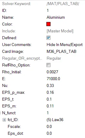
• Import the case 1 rad file, named “Law2_epsmax_failure” and perform the simulation with the law 36 material card. Refer to the video titled "Materials 7" for further information. 

        

Case 7 

• Open the Law27_0000.rad file and perform the simulation with the law 27 material card. Use the recommended shell properties.

Compare 7 cases as discussed in the last 3 slides, in a tabulated format based on:

1. The Total number of cycles, Energy error, mass error, and simulation time.
2. Notice the animation of all 5 and describe the animations in brief based on whether the elements are being deleted or cracked.
3. Plot energies and notice any difference.
4. Based on all the results, which case would represent the on-field scenario.
5. Prepare a ppt/Docx and list down case by case results and your conclusion as to why the failure happened.

PROCEDURE

• Import the model by using  solver deck tool.
• Here we are importing starter file.
• Change the properties and material cards as per the requirments.
• The base simulation is run without any modification to element properties using Radioss option under Analysis tab.(Analysis>radios)
• Create a folder to save the rad files in local directory and edit options providing number of threads as " -nt 4 ".
•  
• After analysis, the .OUT file is viewed to check whether the Energy error and mass error fall within the aceptable range
• The energy error starts from 0% to 10% which is within acceptable range. Mass error stays constant throughout the simulation
• Since the error values are acceptable,internal energy, hourglass energy, total energy of the simulation are plotted with the help of hypergraph 2-D.
• Hyperview is opened to view the simulation . model and results (h3d file) are loaded from the newly created folder.
• Animation shows how the forces affect on the model and simulate the crash propogation.
• To plot the specific graphs, hyper graph 2-d is selected.
• File named end at T01 is opened and specifies energies are plotted against time
• From the plot we will get the energy change throughout the simulation and we canobserve the some result.

     CASE 1

• First import the file FAILURE_JOHNSON_0000.rad into solver
• Here in this there need not change the property card and material card so simulate the model as it is.
• Do the same procedure that explained above with below material card and property card.
• 
• 
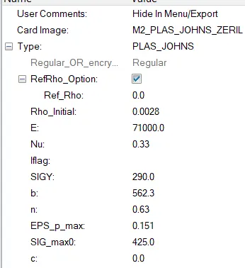
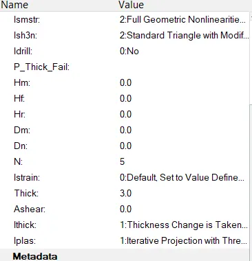
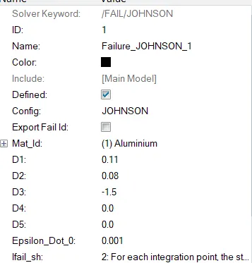
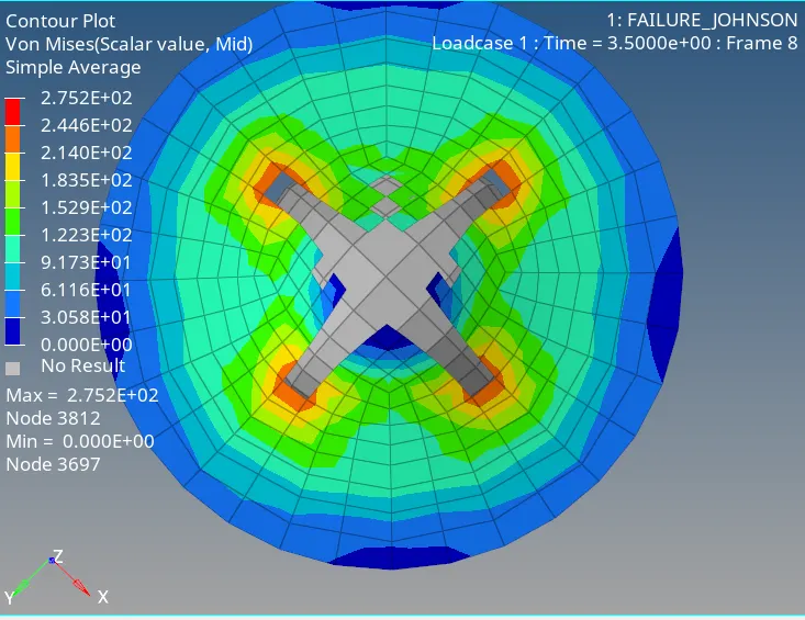
• Simulate the model and save it on supperate folder and open with vonmises stress value.
• Now to run simulation go to hyperview-import h3d file- apply contour - select von misses stress select averaging method as simple - apply
• 
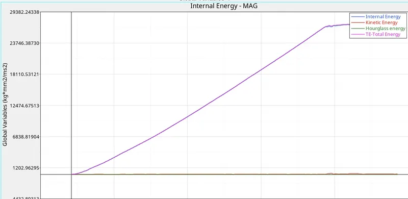
• Plot the graph for energie change
• .
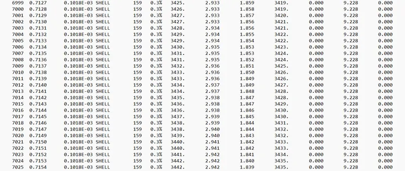
• From ooo1.out file we got energy error and mass error.
• 
• 
• From the simulation we can findout some importent observation:

1. Here energy error is 0.3% which is below 5% so it is acceptible
2. In the simulation ,when the internal stress exceed the youngs modulus by 15% of the material, elements get deleted.
3. From the graph we canfind that internal energy increases until the material get raptured than it go in constant and no Hourglass energy present in the material.
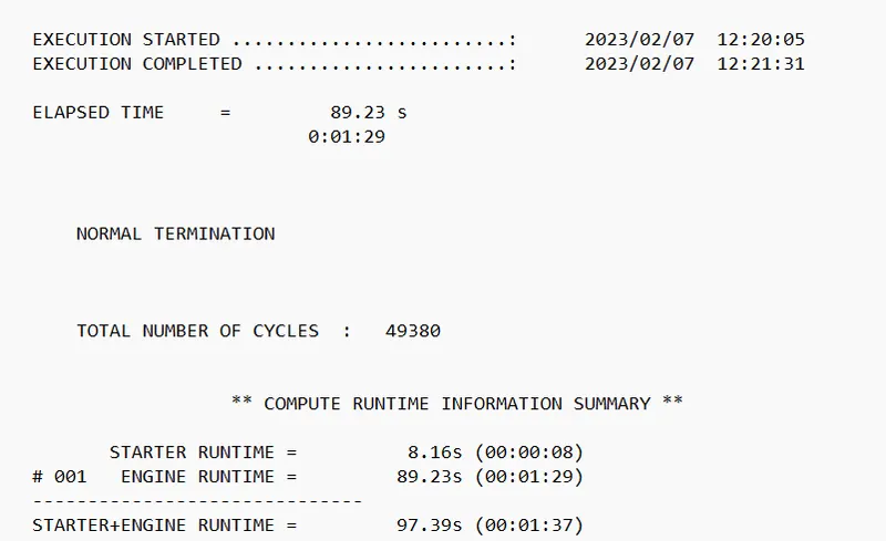
4. Totel no of cycles of simulation is 49380 in 89.23 seconds.

    CASE 2

• First import the file FAILURE_JOHNSON_0000.rad into solver
• Do the similar procedure that we had followed in case 1. But there is some changes in failure card as shown below.
•  
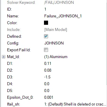
• Here we are addding some values like

                       ifail_sh= 1

                         Dadv= 1

                        Ixfem= 1 

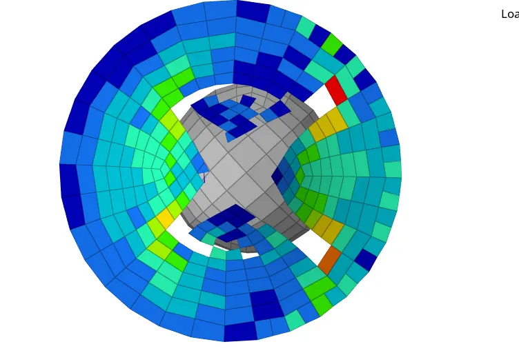
•  As in this case we have set Ixfem=1 this failure criteria will lead to element cracking instead of element or layer deletion
• If the element has no failed neighbour and D-1 then in this case new crack intialization in element
• If the element has failed neighbour and D - Dadv then in this case crack advanced and Dadv used for crack advancement Dadv will be only used if existing crack arrives to a boundary of an element
• Now to run simulation go to hyperview-import h3d file- apply contour - select von misses stress select averaging method as simple - apply
• 
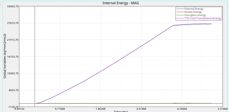
• Plot the graph for energie change
• 
• From ooo1.out file we got energy error and mass error.
• 
• 
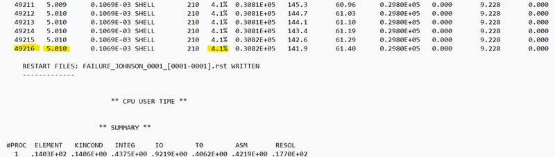
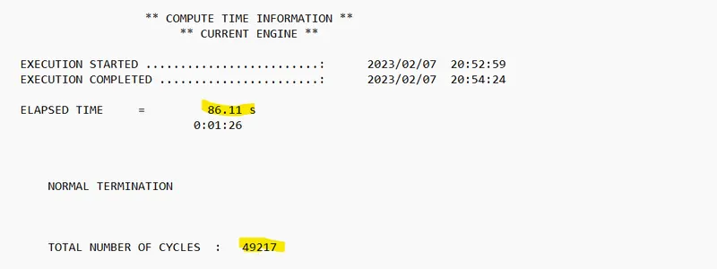
• From the engine file we get energy error as 4.1%.It is acceptible because it is below 5%.
• From the simulation we can findout some importent observation:
  • Here energy error is 4.1% which is below 5% so it is acceptible
  • In the simulation ,when the internal stress exceed the youngs modulus by 15% of the material, elements get cracked and deleted.
  • From the graph we canfind that internal energy increases until the material get raptured than it go in constant and no Hourglass energy present in the material.
  • Totel no of cycles of simulation is 49217 in 86.11 seconds.

   CASE 3

• First import the file FAILURE_JOHNSON_0000.rad into solver
• Delet the failuer card from the smulation and run the simulation.
• 
• 
• 
• 
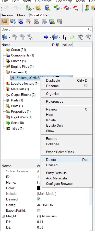
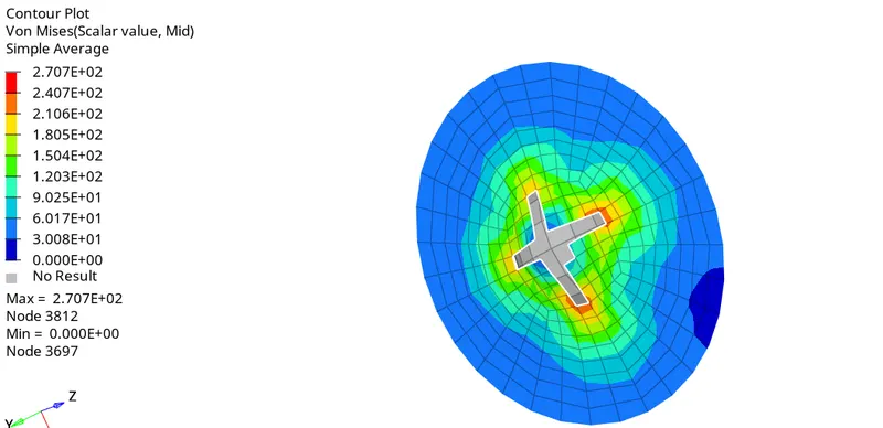
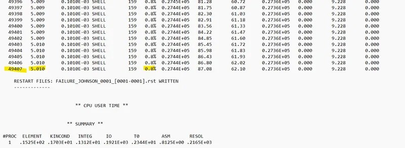
• From the simulation we can findout some importent observation:
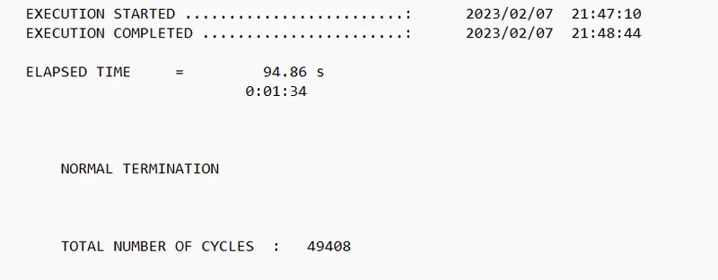
  • Here energy error is 0.8% which is below 5% so it is acceptible
  • In the simulation ,when the internal stress exceed the youngs modulus by 15% of the material, elements get cracked and deleted.
  • From the graph we canfind that internal energy increases until the material get raptured than it go in constant and no Hourglass energy present in the material.
  • Totel no of cycles of simulation is 49408 in 94.86 seconds.

•    CASE 4

• First import the file case 3 starter file into solver
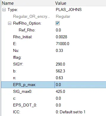
• Now change the materials- Aluminium-set EPS_P_max zero and run the simulation.
• 
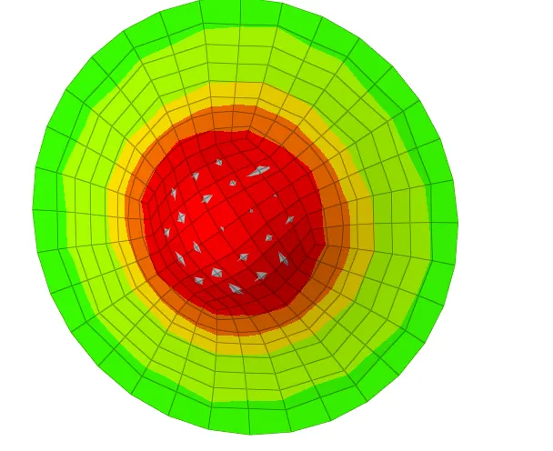
• Now to run simulation go to hyperview-import h3d file- apply contour - select von misses stress select averaging method as simple - apply
• 
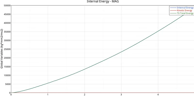
• Plot the graph for energie change
• 
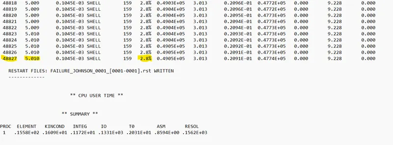
• From ooo1.out file we got energy error and mass error.
• 
• 
• From the simulation we can findout some importent observation:
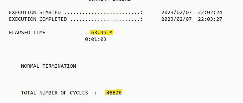
  • Here energy error is 2.8% which is below 5% so it is acceptible
  • In the simulation ,when the internal stress exceed the youngs modulus crack is not happening because we delete the eps_max value.
  • From the graph we canfind that totel energy increases with time because there is no rapture happens.
  • Totel no of cycles of simulation is 48828 in 63.95 seconds.

       CASE 5

• Import the same model in solver.
• Changing the material card from  law 2 (elasto-plastic material) to law 1(linear elastic material)with same values of E (youngs modulus), density and poissons ratio.
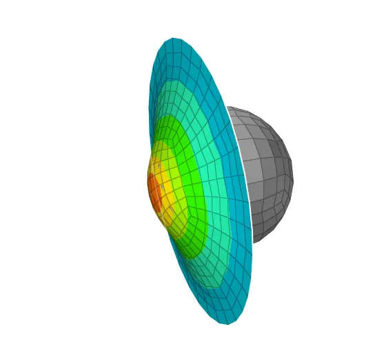
• Now to run simulation go to hyperview-import h3d file- apply contour - select von misses stress select averaging method as simple - apply
• 
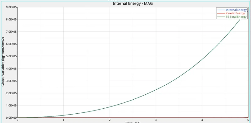
• Plot the graph for energie change
• 
• Check the energy error and time from engine file.
• 
• 
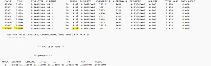
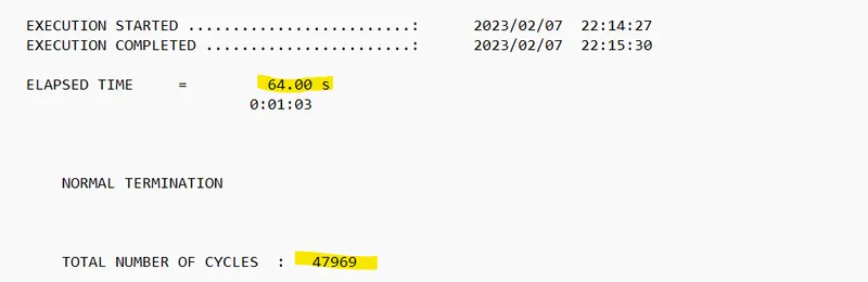
• From the simulation we can findout some importent observation:
  • Here energy error is 1.3% which is below 5% so it is acceptible
  • In the simulation ,when the internal stress exceed the youngs modulus ,there is no any deformation happens.
  • From the graph we canfirmed that totel energy increases with time exponentially because deformation take place in elastic region.
  • Totel no of cycles of simulation is 47969 in 64 seconds.

       CASE 6

• First import the file FAILURE_JOHNSON_0000.rad into solver
• Perform the simulation with the law 36 material card. Give the curve details as shown in the video titled 'Material 7'.
•  
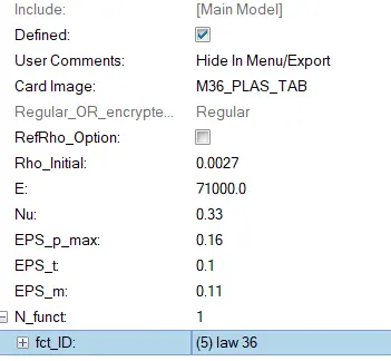
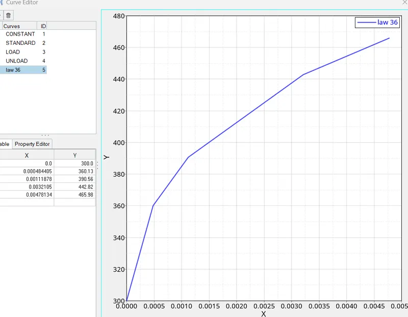
• In this material card, the main advantage is we can add the lab curve directly to the material so we can increase the accuracy of the result.
• Now to run simulation go to hyperview-import h3d file- apply contour - select von misses stress select averaging method as simple - apply
• 
• 
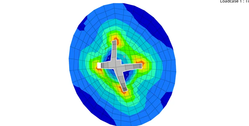
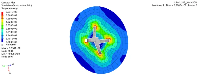
• Plot the graph for energie change
• 
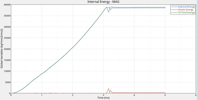
• Check the energy error and time from engine file.
• 
• 
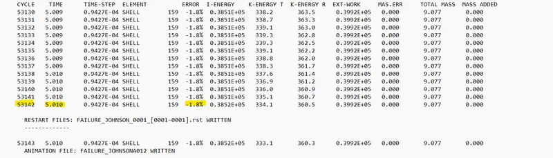
• From the simulation we can findout some importent observation:
  • Here energy error is -1.8% which is below 5% so it is acceptible
  • In the simulation ,when the internal stress exceed the youngs modulus ,there is no any deformation happens.
  • From the graph we canfirmed that totel energy and internal energy increases upto thr rapture and then it goes to constant rate.
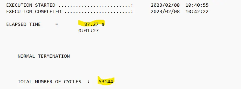
  • Totel no of cycles of simulation is 53144 in 87.27 seconds.

      CASE 7

• First import the file FAILURE_JOHNSON_0000.rad into solver
• We need to use recommended shell properties in this case. Go to Properties > 5NiP. Now, we can look at the utility window and set the following attributes as follows:
  
  I_shell=24, I_smstr=2, I_sh3n=2, N=5, I_thick=1, I_plas=1
• Give material card .
• 
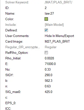
• This law combines an isotropic elasto -plastic Johnson cook material model with an orthographic brittle material failure model .Material damage is accounted for prior  to failure.Failure and damage occur only in tension .This law is only  for shells
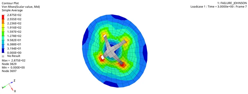
• Now to run simulation go to hyperview-import h3d file- apply contour - select von misses stress select averaging method as simple - apply
• 
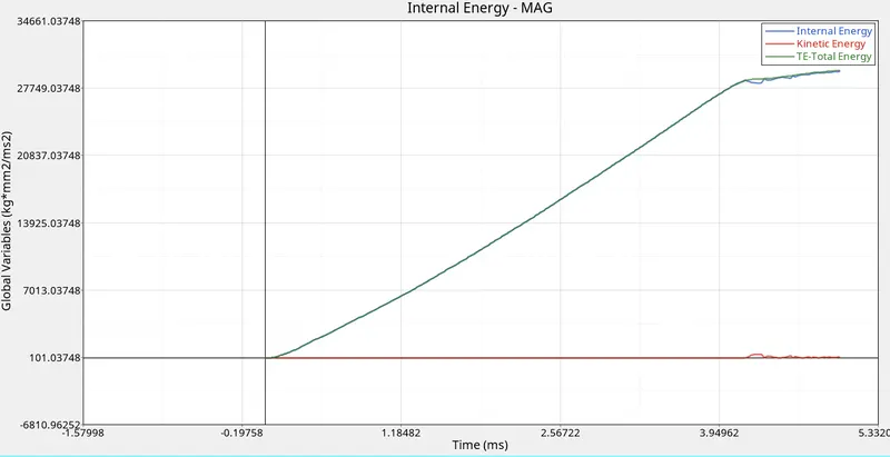
• Plot the graph for energie change
• 
• Check the energy error and time from engine file.
• 
• 
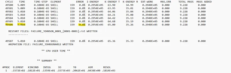
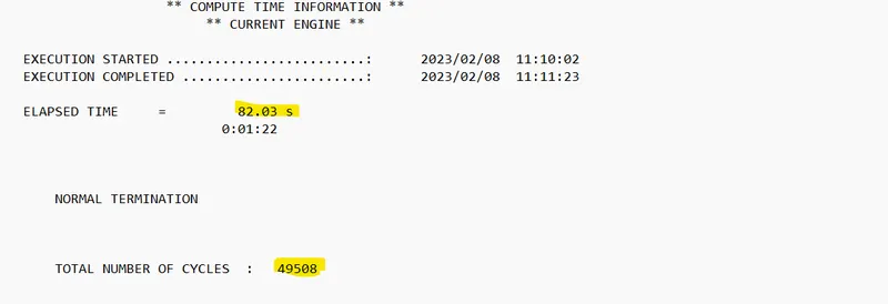
• From the simulation we can findout some importent observation:
  • Here energy error is 0.8% which is below 5% so it is acceptible
  • In the simulation ,when the internal stress exceed the youngs modulus ,material get deformed and deleted.
  • From the graph we canfirmed that totel energy and internal energy increases upto thr rapture and then it goes to constant rate.
  • Totel no of cycles of simulation is 49508  in 82.03 seconds.

OBSERVATIONS

1. CASE 1: In this case, it has the Fail/JOHNSON card as well as EPS_p_max value assigned, with Ixfem value as 0. This means that the elements are deleted as soon as they cross the EPS_p_max threshold, which is what we can see in the above simulation. In this case, it has the Fail/JOHNSON card as well as EPS_p_max value assigned, with Ixfem value as 0. This means that the elements are deleted as soon as they cross the EPS_p_max threshold, which is what we can see in the above simulation.
2. CASE 2: In Case 2 we have used Ifail_sh, Dadv, and Ixfem as part of the Fail/JOHNSON card. Ixfem is especially important here because it decides the way the elements react. With its value equal to 1 here, it means the elements will crack and fail. Along with Dadv, crack propagation can also be seen here, with elements being deleted only when the crack reaches them. As a result, this is a more realistic depiction.
3. CASE 3: With the Fail/JOHNSON card deleted in this case, the onus is on EPS_p_max to be the factor for element deletion. As we can see in the following screenshot, its value is 0.151, meaning elements will be deleted if the strain on any integration point within said elements reaches 15.1% of the plastic strain. The elements, in this case, fail rapidly when compared to the elements in case 2 due to XFEM crack formulation there.
4. CASE 4: The metal sheet is able to withstand a large amount of stress and avoid element deletion primarily due to the fact that the value for EPS_p_max was deleted. Since it was deleted, RADIOSS assigns it the default value of 10^30. In addition to that, the fail/JOHNSON card was deleted. The material behaves like a pseudo-elastic (also called elasto-plastic) material since it has a very high EPS_p_max tand elements cannot be deleted due to no failure cards.
5. CASE 5: In this case, the plate is defined with a LAW-1 material which defines the basic properties of elastic material. This model considers only the elastic phase of the material, there is no plasticity involved which results in linear deformation.
6. CASE 6: In this case we use law 36 material card.Here we can add lab data directly so we get more accurate result.
7. CASE 7: Here we use law 27 material card. In this case the use of the M27_PLAS_BRIT material card that is used for isotropic elastoplastic Johnson-Cook material model with an orthotropic brittle failure model.

CONCLUSION

1. Law 1 material card is mainly used for elastic material. It is used for vibration analysis.This law represents a linear relationship between stress and strain.
2. Law 2 material card  is used in elesto plastic material. We get more realistic approuch in material simulation.
3. Law 36 material card is also used for elesto plastic material. Here we can add lab data directly so it can improve simulation accuracy.
4. Law 27 material card mainly used for brittle materials.