Assignment 4-RADIOSS Material Laws Challenge

Case 1

Import the FAILURE_JOHNSON_0000.rad file and run the model as it is.

intially we are going to import the 0000.rad file and run the simulation on the defaulted values

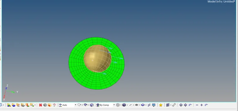
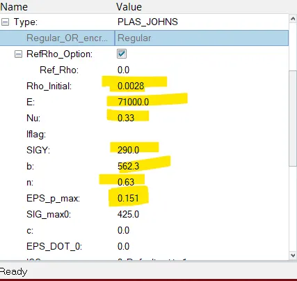
material properties

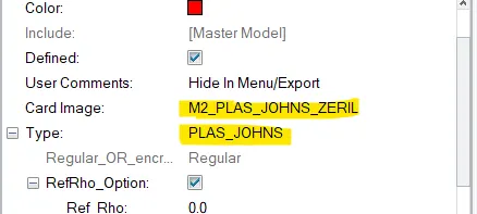
failure card

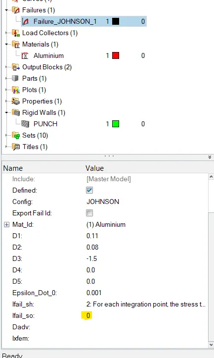
properties

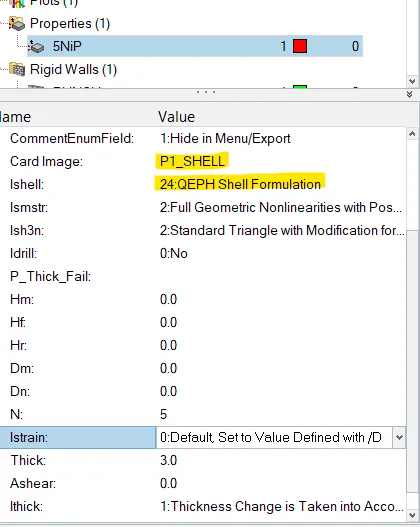
now we are going to run the simulation on defaulted values

click on analysis >click on radioss>save the file as Law2_epsmax_failure.>set option -nt 4 >click on radioss

once we click on the radioss a solver window will open that shows the job completion

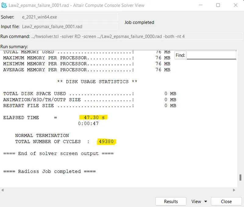
in the above case the the total no of cycles =49380

time taken to complete the job=47.30s

to check the energy error and mass error we need to open the file 0001.out ,in this file we need to scrole down to check the energy error and mass error check

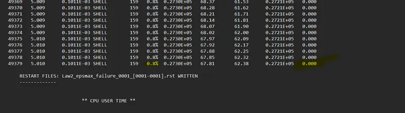
from the above snape the energy errors =0.8%

mass error =0.0%

both the above results are acceptable (-15% to +5%)

the job has been completed now we need to check the results from the hyperview

we can visuvlise the results like von mises stress, displacement,KE, internal energy ,hourglass energy,total energy

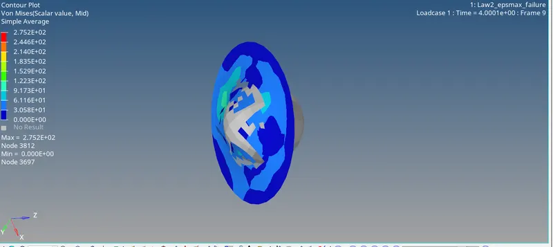
the maximum stress in the component was recorded to 2.75E+02

now to view the results we need to chcek the results in the hypergraph 2D ,for that we need to click on client selector and select hypergraph 2D

in the hypergraph 2D we need to click import the result file that radios solver has generated thats the T01 file

this file will be available in the epmax_p_failure file select T01 file and click on apply a window will open where we need to select the different variables and their magnitude

the variables that can be viewed in the hypergraph window are kinetic energy,total energy,hourglass energy ,R_wall forces and internal energy

case 2

• we Import the case 1 rad file, named “Law2_epsmax_failure” and perform the simulation with failure plastic strain (EPS_p_max) and fail_Johson card enabled.
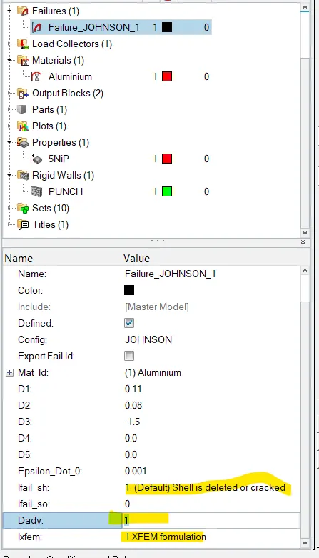
• Changes has to be made in /FAIL/JOHNSON card:

• ifail_sh= 1

ifail_sh =1 it determines whether the shell element will get crack or delete

• Ixfem= 1 taking its value =1 means we have set the condtion for craking ,the element that has been failed while analysis will not get deleted now and crack will propagate further
• Dadv= 1, it determines if the element that factured in the analysis crosses the limit in the fracture or braking in other words if crack goes beyond the limit then the element will fail

to set the values of ifail_sh, Ixfem and Dadv click on the failure card and change the values

now we are going to run the analysis

click on analysis >select Radioss

before going to the analysis save the file as Law2_epsmax_crack

we have saved the file named as law2_epsmax ,now we have to hit the radioss and analysis will get start and it will take few seconds to solver to complete the job

below is the engine file that has generated by the solver ,once the analysis get completed we can see the results

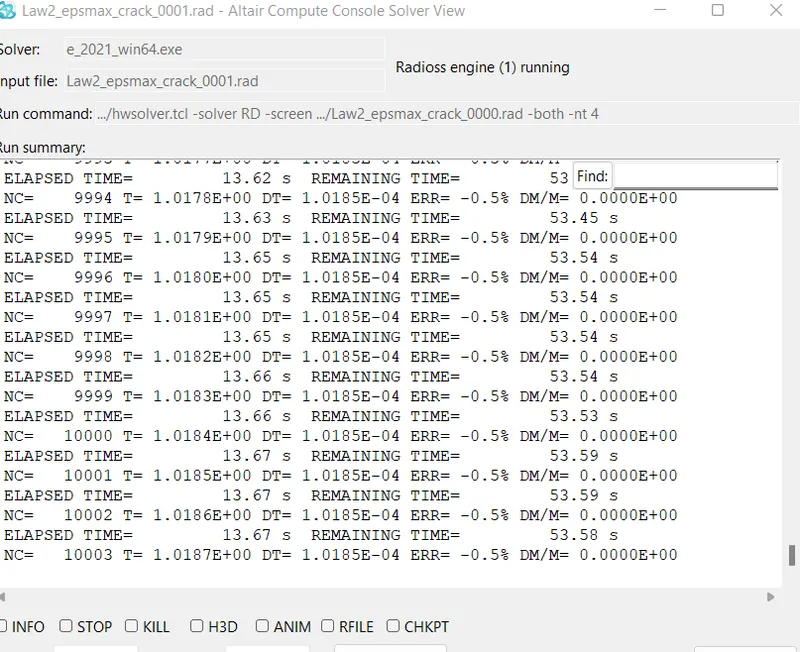
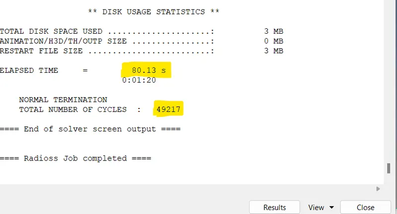
as shown above the time taken in this case is higher than tne first case

time taken=80s

no of cycles =49217

now to check the energy and mass error we are going to open the 0001.out file

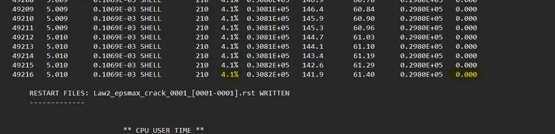
from the above snap the energy error has reached a value of 4.1% and mass error is still 0 therefore these errors are acceptable

we can visuvlise the results like von mises stress, displacement,KE, internal energy ,hourglass energy,total energy FROM THE HYPERVIEW for that we need to input the t01 file from the law2_eps max_crack

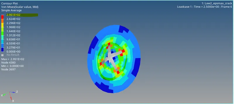
the maximum stress in the component was recorded to 2.951E+02

now to view the results we need to chcek the results in the hypergraph 2D ,for that we need to click on client selector and select hypergraph 2D

in the hypergraph 2D we need to click import the result file that radios solver has generated thats the T01 file

this file will be available in the epmax_p_failure file select T01 file and click on apply a window will open where we need to select the different variables and their magnitude

the variables that can be viewed in the hypergraph window are kinetic energy,total energy,hourglass energy ,R_wall forces and internal energy results will be shown at the end and will compare all the result case

CASE 3

Import the case 2 rad file, named “Law2_epsmax_crack” and perform the simulation by removing the fail_Johnson failure card. Give the title name as Law2_epsmax_nofail.

in this case we are going to import the 0000.rad file from the case Law2_epsmax_crack

once we import this rad file in solver deck we have to click on the model browser ,there is a failure card we have to delete the failure card and we are going to run the simulation with out assining the failure card

below is the image that shows the failure card and we have to right click on it to delete this failure card

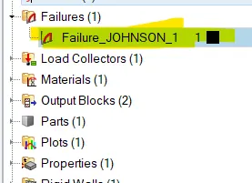
now we have to save the file for that we need to click on save as and save it as law2_epsmax_nofail

now we are good to go to run the simulation

click on the radioss and runn the simulation

a consol window will open for the analysis process once the analysis will get completed the consol window will show the job is complete

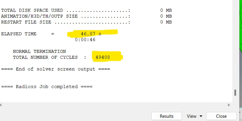
solver takes 46 sec to complete the analysis

total no of cycles =49480 as shown in below snap

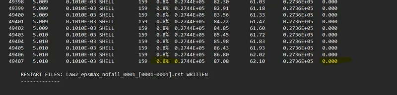
now to check the energy and mass error we are going to open the 0001.out file

the energy error in this case =0.8% and mass error is again 0%

we can visualise the results like von mises stress, displacement,KE, internal energy ,hourglass energy,total energy FROM THE HYPERVIEW for that we need to input the t01 file from the law2_eps max_nofail

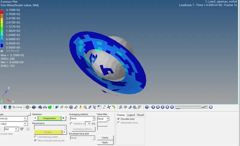
the maximum stress in the component was recorded to 3.109E+02

now to view the results we need to chcek the results in the hypergraph 2D ,for that we need to click on client selector and select hypergraph 2D

in the hypergraph 2D we need to click import the result file that radioss solver has generated ,that is the T01 file .

this file will be available in the epmax_p_nofail file select T01 file and click on apply a window will open where we need to select the different variables and their magnitude

the variables that can be viewed in the hypergraph window are kinetic energy,total energy,hourglass energy ,R_wall forces and internal energy results will be shown at the end and will compare all the result case

CASE 4

Import the case 3 rad file, named “Law2_epsmax_nofail” and perform the simulation by removing both the failure plastic strain (EPS_p_max) and the fail_Jhonson failure card.

In this case we have to import the 0000.rad file from the case 3 save this file in as noepmax_nofail_0000.rad

once we import the file we have to set the epmax=0 and the failure has been already deleted in the last case

process to delete click on material>Set EPS_max=0

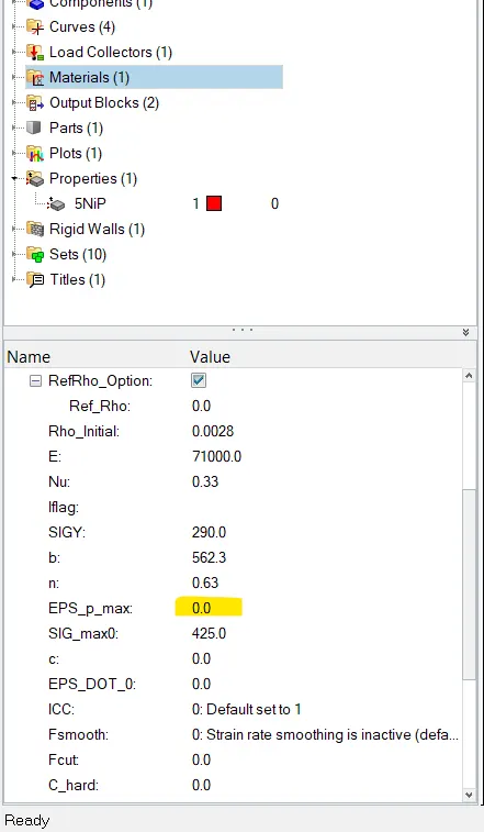
now save the file in a new folder named case 4 and file name noepsmax_no fail.0000.rad

now we are good to go for simulation click on radioss and analysis will get start this can be viewed from the consol window shown below

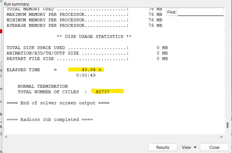
time taken by the simulation =49.sec

total no of cycles =48737

now to check the energy and mass error we are going to open the 0001.out file

the energy error in this case =3.1% and mass error is again 0%

as shown the energy and mass error are within acceptable range

we need to check the results from the hyperview

we can visuvlise the results like von mises stress, displacement,KE, internal energy ,hourglass energy,total energy

in the hypergraph 2D we need to click import the result file that radioss solver has generated ,that is the T01 file

this file will be available in the no_epmax_p_nofail file select T01 file and click on apply a window will open where we need to select the different variables and their magnitude

the variables that can be viewed in the hypergraph window are kinetic energy,total energy,hourglass energy ,R_wall forces and internal energy results will be shown at the end and will compare all the result case

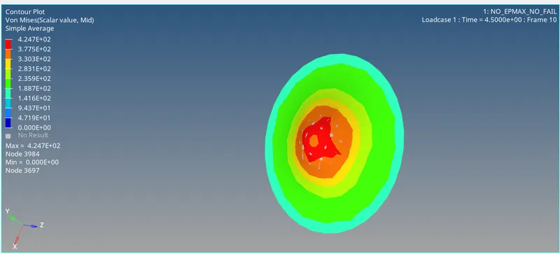
all the results will be discused at the end

Case 5

Import the case 4 rad file and perform the simulation by changing the material card to Law 1. Keep the same value for rho, E, and nu values.

in this case we need to change the material card to law 1

the law 1 is material card for elestic model in this we are expecting the maximum stress absorpton

import the solver deck /0000.rad file from the case 4

now we need to change the material card

click on the material card >set card image =M1-ELAST>set rho_intial=0.0028, youngs moduls E=71000 and poisions ratio nu=0.33 below is the snap after changing the values

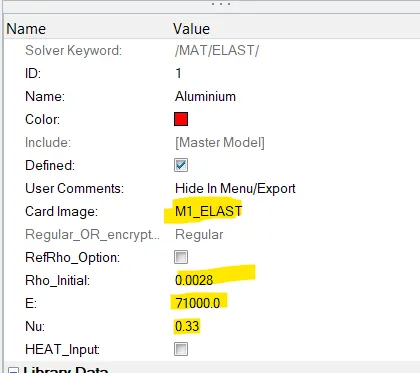
now we are ready for the analysis before analysis save the file in different folder name it as LAW1_M1-ELAST

Click on radioss a consol window will open to show the compelation of job

from the below snap the job has been completed ,the solver takes 49 sec to complete the job

total no of cycles=47969

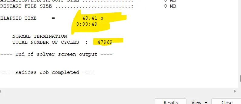
now we are going to check the mass and energy error check ,to check energy we need to open the 0001.out file from the file folder of this case

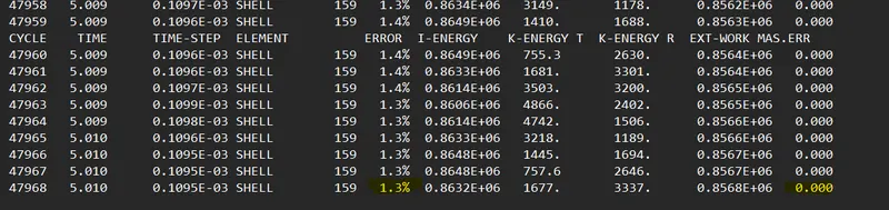
from the above image the energy and mass error in this case is 1.3% ,0.0% and which is acceptable

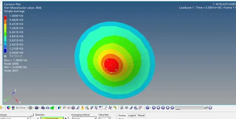
in order to view the results we need to go to the hyperview where we can see the results like displacement ,von-mises stress ,

for that we need to import H3D file from the file folder of case 5

proceduure

click on client selector >select the hyperview as shown below

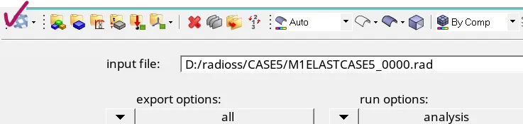
after open the window of hyperview we need to input the h3d file from the file folder and click on apply

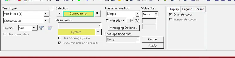
now click on contour option from the tool bar >from the result type select von mises >averaging method=simple>select component>click on apply

now play the animation

CASE 6

Import the case 1 rad file, named “Law2_epsmax_failure” and perform the simulation with the law 36 material card. Refer to the video titled "Materials 7" for further information

import the 0000.rad file from the case 1

after importing the solver deck file we need to change the material card and this can be changed from the model browser

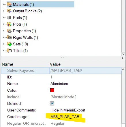
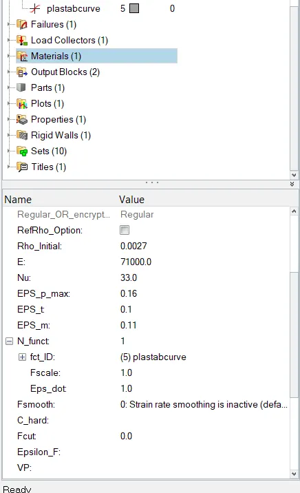
click on model browser >click on material>change the card image as M36_PLAS_TAB

Now we need to assign the material properties

we have taken the values from the video as shown below

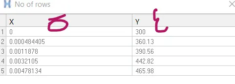
now we need to create a function ID this is the case were user can define it own streess and strain value

to create the curve we need to click on the curves in the model browser and right click on it a window will open we have to hit the create option ,we named this curve as plastabcurve

now set the stress and strain values in the X,Y table

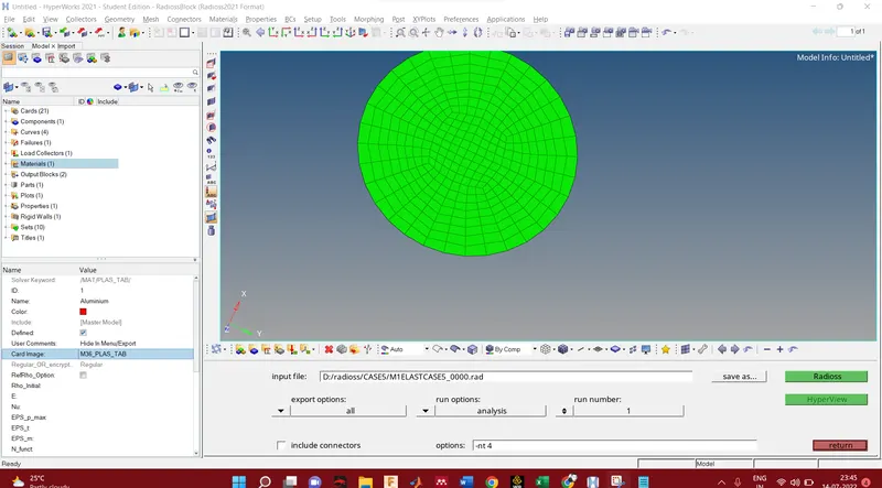
before analysis we are going to save the file as LAW36_PLAS_TAB

now we are ready to go for analysis

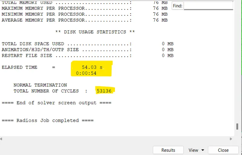
analysis has been completed as shown below

time taken =54sec

total no of cycles=53136

now we need to check the energy and mass errors for that we need to open 0001.out file

from the below image both energy and mass error are within the acceptable range

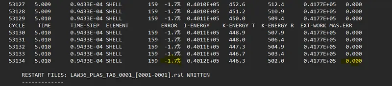
we can visualise the results like von mises stress, displacement,KE, internal energy ,hourglass energy,total energy

\

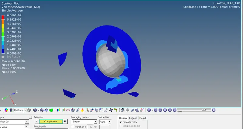case 7

Open the Law27_0000.rad file and perform the simulation with the law 27 material card. Use the recommended shell properties.

This law models an isotropic elasto-plastic material using user-defined functions for the work-hardening portion of the stress-strain curve (for example, stress vs. plastic strain) for different strain rates

change the card image to m36_plas_tab

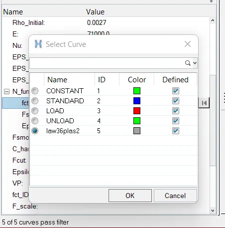
change the values of rho,E,EPS_P_max, below are the parameters that has been changed

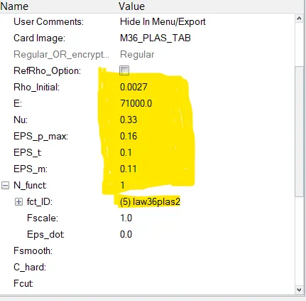
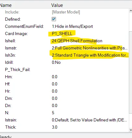
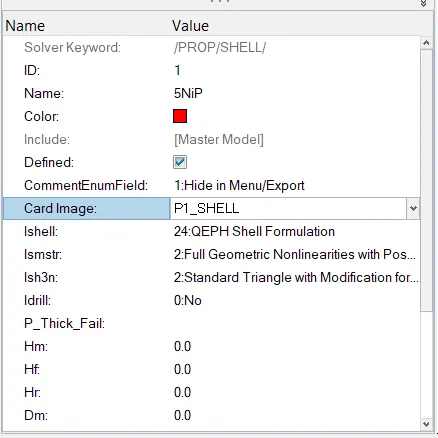
to change the properties as shown below we need to click on the property>click on 5NiP

NOW CHANGE THE SHELL ELEMENT FORMULATION

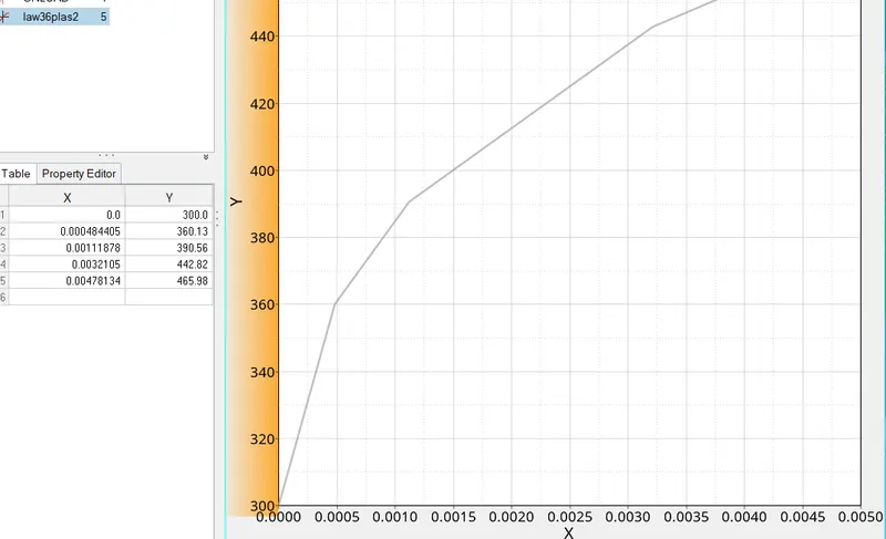
to create the curve we need to click on the curves in the model browser and right click on it a window will open we have to hit the create option ,we named this curve as plastabcurve

now set the stress and strain values in the X,Y table

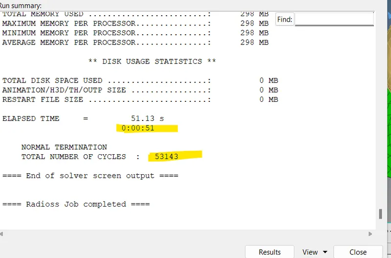
the job has been completed

total time taken =51 sec

total no of cycles

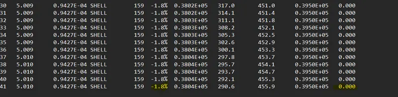
lets check the energy and mass errors

both the errors are within acceptable range

to analyse the stress in the component we need to go to the hyper view ,we need to input the H3D file from the file folder of this case

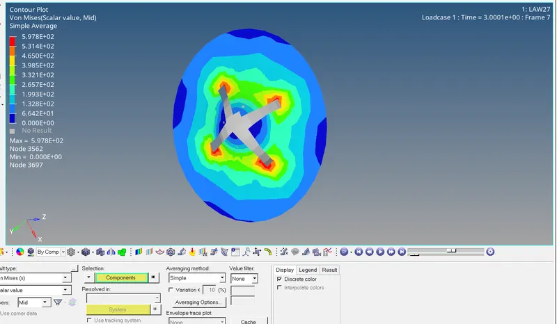
the stress value has reached to a maximum value of 5.978E+02

lets discuss the results of all the cases

case 1

in this case johnson failure card has been used and eps_max value has been assigned

the eps_max value has taken =15%

ixfem=0

the meaning of the above values is that when the element reaches the plastic strain value of 15 % the element will get delete or crack

if the ixfem value has take=0 the element will get delete once it reaches the epsmax=15%

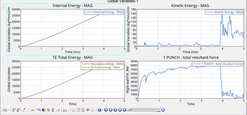
from the 2d plot below it is clearly shown the internal energy increases upto the 4 sec and after that the internal energy remains constant this means that the component has stored lot of energy upto 4s or we can say maximum displacement has occured and after 4 sec the steady state comes into picture which means there is some reactive forces which is being applied to the rigid sphare.

kinetic energy : the rigid sphare is going to hit the component at 0.5 sec you see a sudden peak in the KE plot at o.5sec .at 4sec the more force has been applied to the component at this time and you can see the sudden peak of KE at 4.sec after 4 sec the elements are getting deleted from the component you can see the fluctuation happening both in the rigid wall and kE plot

when lot of elements got deleted from the component which are in the path of rigid sphare you can see the drop of rigid wall forces from the plot below .there are not many elements that can oppose the rigid sphare .

the hourglass is almost zero as we have used shell element formulation in this case =shell24 has been assigned to control the hourglass effect

CASE 2

In this case we have enabled the johnson failure card and eps_max , in the case first we set the value of ixfem =0 but in this case its value can be taken 1 which will give us clear idea about the delete and cracking of the element in this case the element get delete only if that element violate the threshold limit.

in this case we are going to activate the below

• ifail_sh= 1
• Dadv= 1

from the below plot if we compare this with the first case

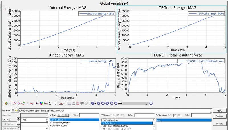
internal energy increases linearly beyond 4sec thus we can say lot of energy has been absorbed by the component hence the displacement will be more to that of the case 1

from the rigid wall forces plot the Rwall force increases upto the 3.8 sec the rigid sphare pushs the component upto its limits when the r_wall crosses the limits then elements either get delete or crack in the path of rigid sphare thats why the rwall froces decreases after 3.8sec because there are not enough elements to push back the rigid sphere.

from the kinetic energy plot at 3.8 sec there is requirement of addtional force for the rigid sphere thats why the the component gets deformed upto its limits and after that increasing some addtional force will results in the deletion of element

CASE3

in this we have deleted the jhonson failure card but keeping all the parameters as it is epsmax values has beel assigned

there is only eps_max value that can deside the element will get fail/delete if the strain goes beyond 15% and the element will delete

taking xfem into consideration the crack will propragate quickly and henc the deleting of element will be very quickly

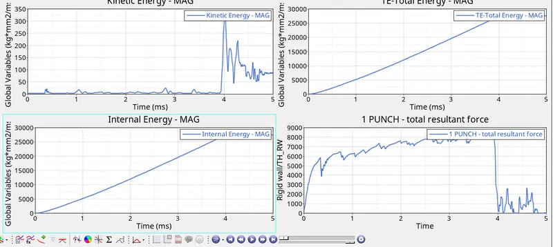
from the plot below the internal increases linearly upto few seconds and after that the component gets stiffer and need some more energy to deform the component thats why you can see from the KE PLOT there is increase in kinetic energy

once the elements reaches above the eps_max value the elements are going to fail ,also from the rigid wall forces these forces also get decreased very quickly becoz the elements that came into the path of rigid spher got fail very quickly

case 4

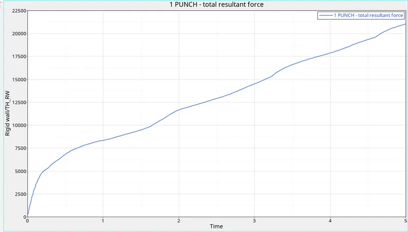
Law 2 (PLAS_JOHNS) expresses material stress as a function of strain, strain rate and temperature.

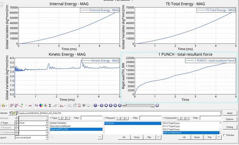
The metal sheet is able to withstand a large amount of stress and avoid element deletion primarily due to the fact that the value for EPS_p_max was deleted. Since it was deleted, RADIOSS assigns it the default value of 10^30. In addition to that, the fail/JOHNSON card was deleted. The material behaves like a pseudo-elastic (also called elasto-plastic) material since it has a very high EPS_p_max threshold and elements cannot be deleted due to no failure cards.

With the value of c (Strain rate coefficient) = 0, there is no strain rate (neither does temperature play a role here). As a result, the stress, in this case, is purely a function of strain generated in the material.

Added, the kinetic energy generated in this case is almost negligible compared to the internal (and total) energy here. The total energy increase is almost linear over time.

Case 5

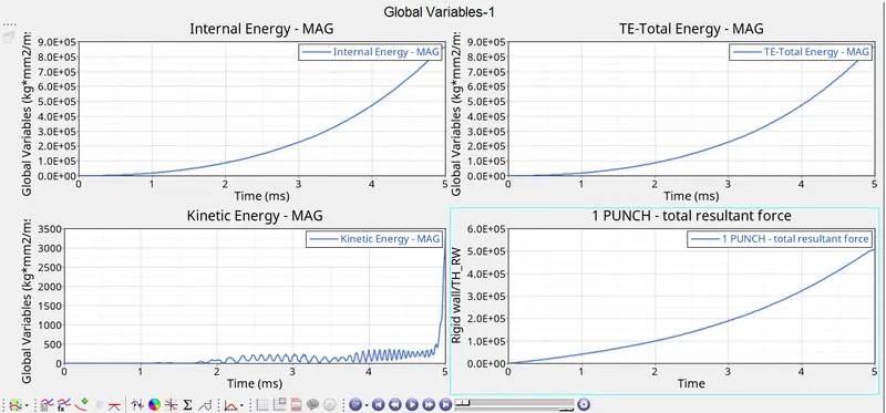
in this case we have use the elastic material law model that is LAW 1

in this case the case the component is going to absorbe sufficent energy and there would not be any element deletion because of elastic property

in this model we are only focusing on the plastic region

from the the plots below the total energy internal energy and R_wall forces increases significantely this is due to the elastic nature of the component

case 6

LAW36 PLAS_TAB

This law models an isotropic elasto-plastic material using user-defined functions for the work-hardening portion of the stress-strain curve (for example, stress vs. plastic strain) for different strain rates

case 7

This law combines an isotropic elasto-plastic Johnson-Cook material model with an orthotropic brittle failure model. Material damage is accounted for prior to failure. Failure and damage occur only in tension. This law is applicable only for shells.

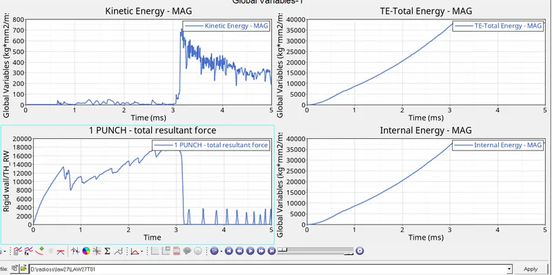
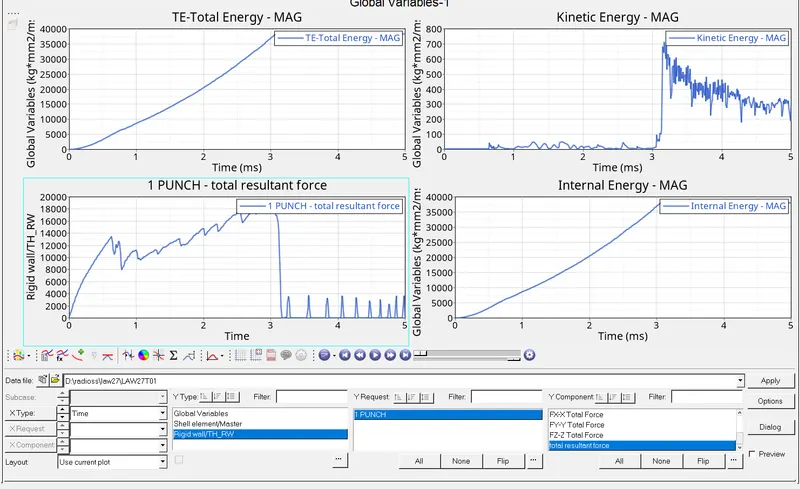
In this case, from the simulation, we can say that this material exhibits strong brittle behaviour. It does not bend as much in response to the applied force and immediately disintegrates. There seems to be not much cracking and the region of element deletion takes the shape of the sphere. Another thing that we can notice is that the stress concentration is localized around the region of impact and these stresses are not dissipated throughout the whole metal plate.

On the topic of energy wastage and element deletion, it is more particularly visible in the rigid wall force graph. Each of the spikes is due to an element deletion. The resultant force gradually increases past the same 3ms mark which is when the sheet gives way and lets the sphere through. With not much of the sheet in the way, the rigid wall forces are drastically reduced, and that results in that drop at the 3ms mark. The first drop occurs when the sheet ruptures the first time.