Assignment 4

Characterizing and understanding the behavior of elastic (Law 1), Isotropic elasto-plastic (Law 2 and different cases, Law 27, Law 36) material.

Introduction:

Elements are the way of representing the CAD model infinite form. Then we take the modeled elements to perform the simulation. Now, the elements themselves do not have material characteristics. So, we define the material properties of those elements to gain proper results. There is a different material card made for different materials and they are expected to behave accordingly. Hence, it leads us to grasp the knowledge about the material cards and understand so that we can implement for our choice of material.

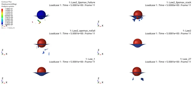
                 In this paper, we will be discussing these many cases as shown below:

Law 1	Case 5	Linear elastic material, Isotropic, for small deformation
Law 27	Case 6	Isotropic elastic-plastic material (Johnson-cook)	ORTHOTROPIC BRITTLE FAILURE, FAILURE IN TENSION ONLY
Law2	Case 1		EPS_MAX, FAILURE CRITERIA
	Case 2		EPS_MAX, FAILURE CRITERIA (Ifxem is activated)
	Case 3		EPS_MAX, NO FAILURE CRITERIA
	Case 4		NO EPS_MAX, NO FAILURE CRITERIA
Law36	Case 7		USER DEFINED FUNCTION FOR HARDENING STREE-STRAIN CURVE

Now, we will elaborate on the simulation process and results obtained with comparisons. The discussion is made on a material law basis:

Aluminum metal is used for the comparison basis. The elastic modulus used for the analysis is 71 GPa. Before performing analysis of the different case, knowing yield strength and ultimate strength will be very handy:

For Aluminum with E= 71 GPa:

Yield Strength: 290 MPa

Ultimate Strength: 425 MPa

Law 1 (Elastic material property card, Case 5):

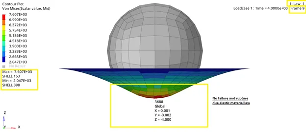
This material is elastic and does not possess any non-linear behavior. It means even if the material is failing then it will be not crack or damage. Thus one has to probe clearly where the stress level has reached beyond the ultimate/ yield strength in order to decide whether the system had failed or not.

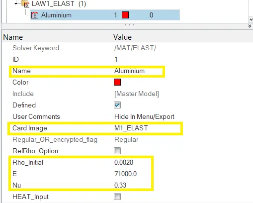
The material properties for this law are shown below which is an ALUMINUM with defined density, elastic modulus, and Poisson's ratio. No other option is available like failure criteria, hardening, and integration point because this material never goes under the non-linear elastic/ plastic zone.

 

Law 2 (Isotropic Elastic-plastic material, Case 1-4):

Law 2 which is Johnson-cook material for elastic-plastic material is studied for four different cases by tweaking the value. Let's see each case for law 2 material:

• Case 1:

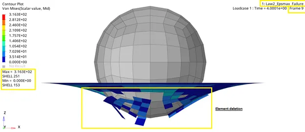
This material card (Johnson cook material, law 2) considers the non-linear effect of the material. So, whenever material reaches the value of yield strength, material deformation will be considered non-linear. As the stress reaches the point of ultimate strength it will be deleted.

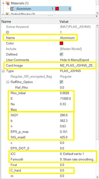
In this material, SIGY which is yield stress is given 290 MPa and SIG_max0 is 425 MPa. The most important thing is Iflag which provides us the choice to enter the material tested value for the non-linear effect. In this case, the Iflag is set to default which means we have to enter the value for yield stress, plastic hardening exponent (n) and parameter (b).

                                             Strain rate effect: The activation and deactivation of this effect is controlled by strain rate co-efficient (c) and reference strain rate (EPS_DOT_0). If you set c=0 or EPS_DOT_0 = high enough not to reach (like 10^3) then effect of strain rate will be not considered.

                                             Effect of strain rate on SIG_max0: ICC flag is useful if one wants to see the effect of strain rate on maximum stress value. It is possible to account for the effect of strain rate over yield region only or over the entire non-linear region starting from the yielding point. In this case, the ICC value is set to default which means the strain rate is taken into account over the whole region. Again, if we look back then we will see the value of c is set to 0 thus strain rate is no longer in action, and the value of ICC will be ignored.

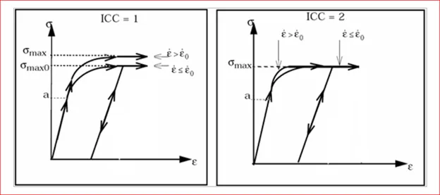
Figure depicting the effect of strain rate over sigma maximum (courtesy: Altair Hypermesh)

The failure model used in this case is the Johnson cook failure model.

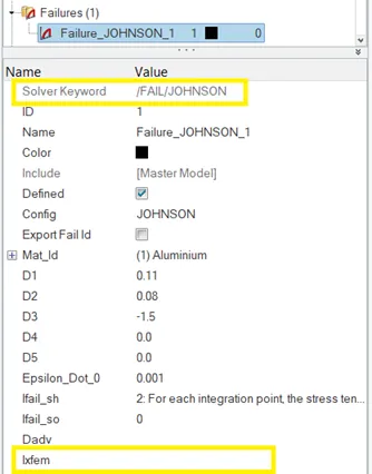
Fail Johnson model is used for a ductile material. It requires data relevant to plastic strain to compute the failure during plastic deformation. The D parameter is used for calculating stress triaxiality which indicates the dominant mode of deformation (shear, compression, or tension).

                              Ifail_sh is crucial if you've defined a number of integration points (N) in the physical properties of the element. Ifail_sh suggests the algorithm whether to delete the element or not when the given threshold stress value is reached. Actually, when the number of integration points is only one then the element will be deleted/cracked (delete or crack option is governed by Ixfem) whenever threshold value is attained. But when a number of integration points is higher than the threshold value is calculated for each integration point. If anyone's integration point is below the threshold value then no deletion or crack will be incurred.

                              Ixfem shows how the element should be deleted once the threshold value will be attained. From here you will decide whether the element should be deleted or cracked.

In this case the Ifail_sh value is 2 and Ixfem is set to default which means the element will fail only when all the integration point has reached the threshold value and the failure will happen by deleting the element.

• Case 2:

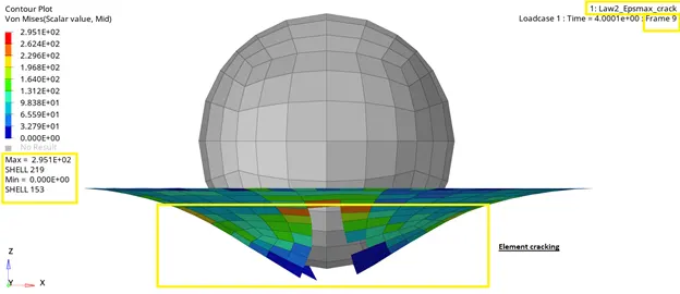
This is the same as case 1. The only difference is in Johnson failure criteria where the value of Ixfem is changed to 1. This means the element is going to crack instead of delete.

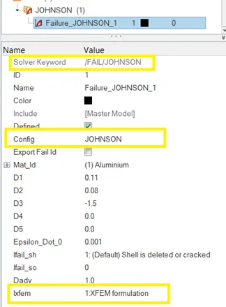
• Case 3:

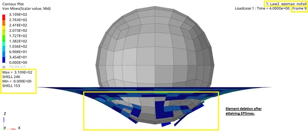
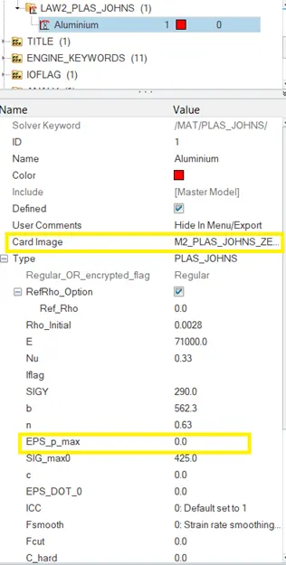
In case 3, the failure criteria are excluded from the consideration and only Law 2 is kept with EPS_max_0. So, despite that, the failure of the element will be computed using the default method called maximum principal strain. The element will be deleted only when maximum EPS_max_0= 0.151 mm will be reached.

 

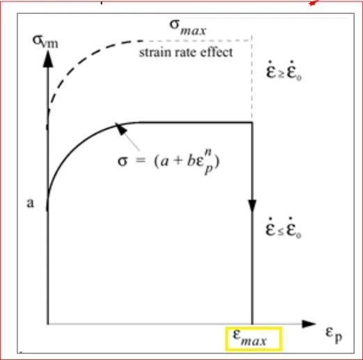
Failure occurring at maximum principal strain (Emax)

• Case 4:

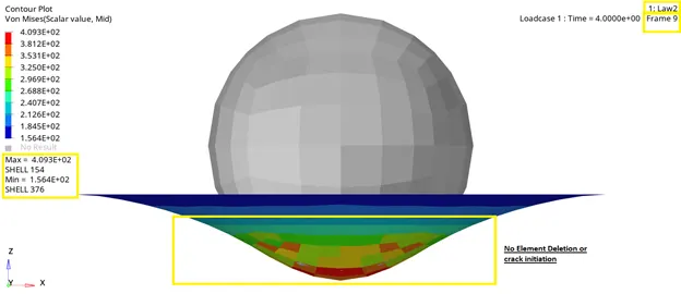
In this case, we will set the value of maximum elastic-plastic strain (EPS_max_0) to 0. This means we have no criteria which will detect if element failure occurs. Hence, elements keep elongating without any failure. Let's have a look at the material card:

Law 27 (Brittle damage: Johnson cook plasticity model, Case 6):

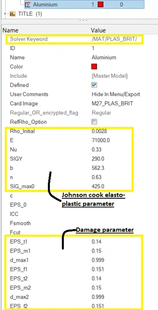
This model is used for the material which undergoes orthotropic brittle failure/damage. This is an isotropic elastoplastic material and to consider brittle failure, the damage phase is joined to the last part of the elastoplastic stress-strain curve as shown in the figure. The damage parameter in this material law is tensile rupture strain (crack initiation), maximum tensile strain, maximum strain for deletion of the element, and damage factor which decide how damage initiates and propagate and how the element will be deleted and how much stress will be reduced. In case if there is multiple integration points and anyone integration point reached the maximum threshold value of maximum strain then the element will be deleted unlike Law 2.

               So, the damage parameter is the only things that are different from other Johnson cook material and help simulate brittle failure in orthotropic direction.

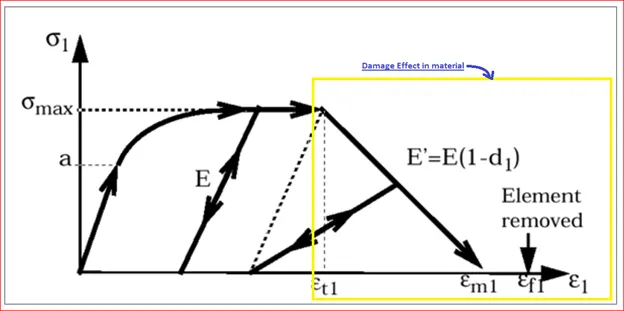
Stress-strain curve including damage effect in the material

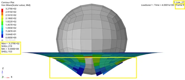
This material law is the same as Johnson cook but incorporates damage parameters to simulate the failure of the material. The failure of the element will be simulated for tensile load only. The damage parameter should be given for two orthogonal directions as shown in the material card because material behavior is different for orthogonal direction:

Law 36 (Isotropic Johnson cook material with user-defined hardening function, case 7):

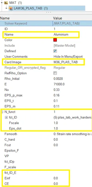
This material law is much more alike Law 27 in terms of damage parameter and calculation and follows the same algorithm when strain failure initiates. The huge difference is the hardening portion of the stress-strain diagram. The hardening portion has complex behavior so more often we supply experimental data to predict the more accurate behavior. The data (fct_ID) is given for different strain rates in ascending manner. The other important parameter is fct_Ide, Eint, Ce. These parameters help in calculating the young's modulus while unloading (spring back).

In this law, once the maximum plastic strain is reached even at one integration point then the failure of the element will occur. In our case, the number of function identifier enter is only one where one can give as many as function identifier data for the corresponding strain rate.

In this case, Young's modulus is kept constant as there is no spring-back action that's why the value of Eint, Ce, and Fct_Ide is kept zero.

Results and Discussion:

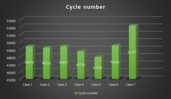
From the above bar chart, we can say that that the simulation time is higher for Case 7 which is Law 36 (Johnson cook tabulated) whereas the number of cycles is less for Case 5 which is Law 1 (Linear elastic material). The number of cycle for each case for Johnson cook isotropic elastoplastic (Law 2) material is almost the same with some differences.

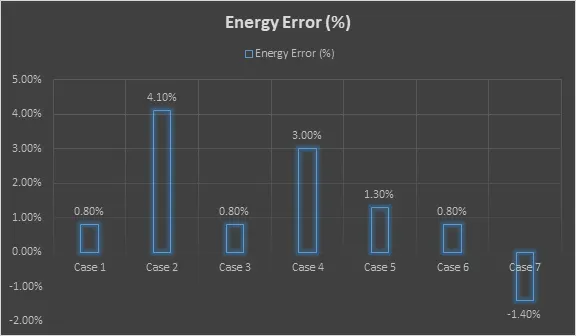
The acceptable positive energy error is 1-2% but in Case 2 (Law 2) and 4 (Law 4) the error is above the given threshold value which must be revised. In case 2 energy error might have had occurred due to the activation of Ixfem. In case 4 the energy error might have had occurred due to the deactivation of elastic-plastic strain which lefts no mean to cause failure when failure strain is reached.

The acceptable range of hourglass energy error is 10- 15 % so the negative error occurring in case 7 (law 36) is acceptable.

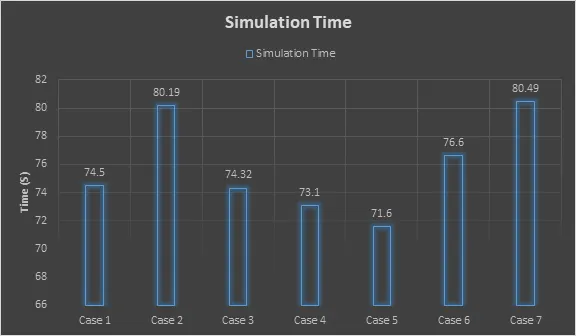
The simulation time chart table is showing that the simulation time required for Case 7 is higher than Case 2 than Case 6 and then case 1 and so on. The case 5 (law 1) linear elastic material is showing good performance with respect to time. As Case 7 uses user-defined material and also due to negative energy error, simulation time has increased. In case 2, the activation flag Ixfem in the Johnson cook failure model might have increased the computation time for crack.

Now, let's talk about the Internal energy of the system for different cases:

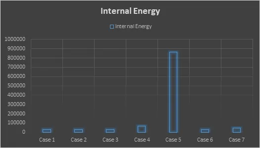
From the above bar diagram, you can see that the internal energy is so high in case 5 which is due to the linear elastic property. Indeed, in this case, the element never goes under failure or damage hence all internal energy keeps piling up and so is true for case 4.

Have some insight from von-misses stress and animation:

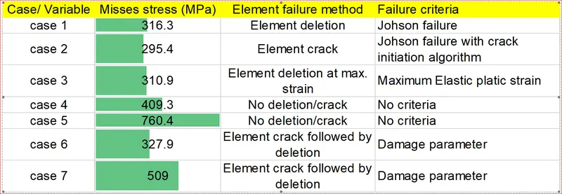
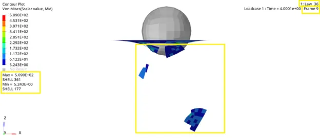
As aluminum is a ductile metal and failure is assumed at the yield point is reached. Here, every case has reached the stress up to yield but cases 4, 7, and 5 went beyond the ultimate strength of the metal. Despite that element, damage has no occurred in cases 4 and 5.

Learning Outcomes:

• Significance of selecting the proper material card for simulation
• Analyzing different materials on the basis of internal energy, stress, and animation.
• The behavior of Johnson cook material in different forms
• Significance of failure criteria

Conclusions:

From the above discussion, we come to conclude that case 1, 3, 6 and 7 show the best result in terms of energy error and failure method. Out of this, case 3 (Johnson cook law with eps max) has shown the best result in terms of internal energy and crack initiation and time.