RUPTURE PLATE SIMULATION CONSIDERING 7 DIFFERENT CASES

AIM : To compare the results of simulation with 7 different cases on RUPTURE PLATE by plotting the graphs and tabulating the result.

OBJECTIVE :

here in this challenge we are going to run the model with different material laws and criterias as follows

• 1. we run the simulation by using Failure johnson model and named as Law2_epsmax_failure and save the results.
• 2. By modifying the failure johnson parameters of previous model such as Ifail_sh,Dadv,Ixfem and named as Law2_epsmax_crack.
• 3. By deleting the Failure johnson card and run the simulation as Law2_epsmax_nofail.
• 4. By deleting the Eps_p_max value and run the simulation as Law2.
• 5. By changing the card image of previous model from Law2 to Law1 Elastic and save the results.
• 6. Again change the card image of previous model from Law1 to Law36 Elasto_plastic and save the results.
• 7. Importing the Law27 model with recommended shell properties and run the simulation.

then we will observe the changes by plotting the graphs for each case then we tabulate the results and made some decisions

PROCEDURE :

CASE 1 - LAW2_EPSMAX_FAILURE :

This case is carried out by using M2_PLS_JOHNS_ZERIAL (MAT/LAW2/(PLAS_JOHNS))

• Isotropic Elasticity

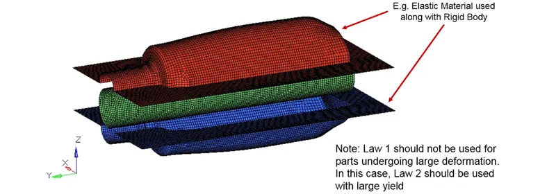
This keyword /MAT/ELAST defines an isotropic, linear elastic material using Hooke’s law. This law represents a linear relationship between stress and strain. It is available for truss, beam (type 3 only), shell and solid elements.

Useful for elements attached to rigid body.This material law is used to model purely elastic materials. The material stiffness is determined by only two values: the Young’s modulus (E), and Poisson’s ratio (n). The shear modulus (G) can be computed using E and n, as shown below:

`G=E/(2(1+nu)`

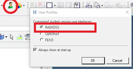
After opening hypermesh we will change the profile to RADIOSS,or we can change it manually by clicking on the profile button marked in red circle in the below picture.

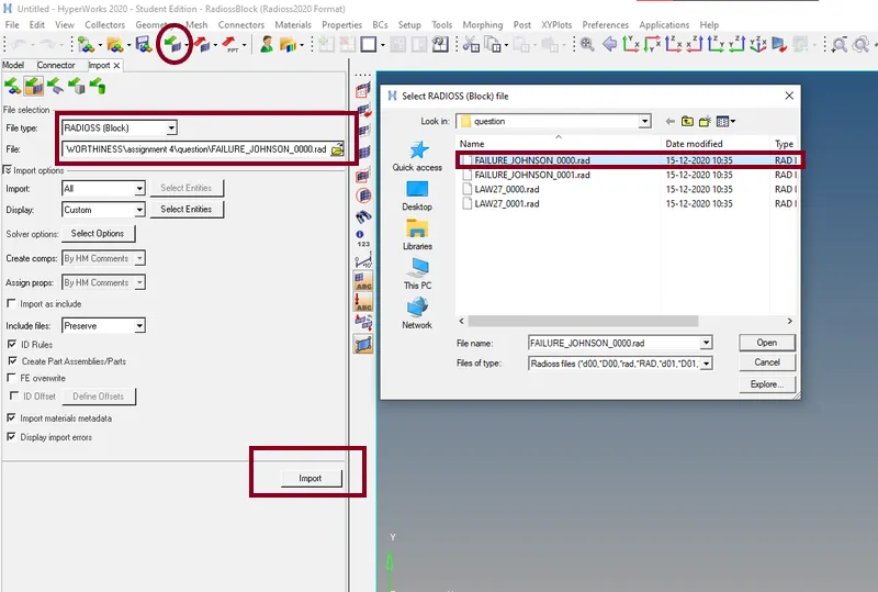
then we will import the engine file we got from the assignment by clicking on "import solver desk" () button available on the top.then we will be redirected to import tab where we will import the file type: filename.rad from the folder where we have downloaded the model.after importing we can see the model appears in wireframe mode which we can turn it into shaded mode.

to check the properties shift to "model" Tab there we can see all the components, properties,curves,materials etc., in which we will check for the properties of the material .from the below image we can see that the model is of aluminium material with material card M2_PLS_JOHNS_ZERIAL

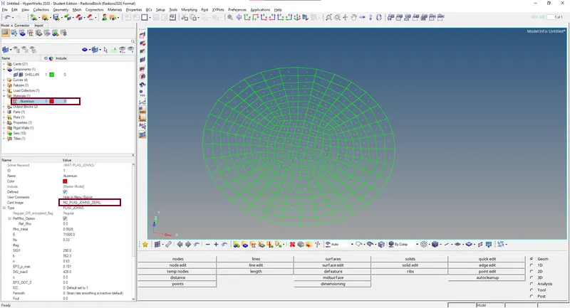
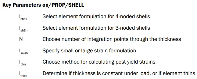
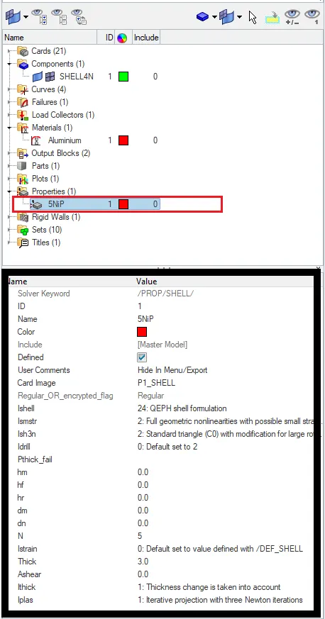
and when we click in the properties we can see that it is having /PROP/TYPE1 or /PROP/SHELL formulation with the following shell parameters.before we proceed with the simulation lets see what are these formulations and properties in detail.

/PROP/TYPE1 or /PROP/SHELL: QEPH

• QEPH is an improved under-integrated 4 node element with 1 integration point on the surface
• Physical hourglass stabilization
• Best compromise between cost and quality
• Generally, QEPH elements costs only up to 15% more than a BT element and the results are close to those of QBAT

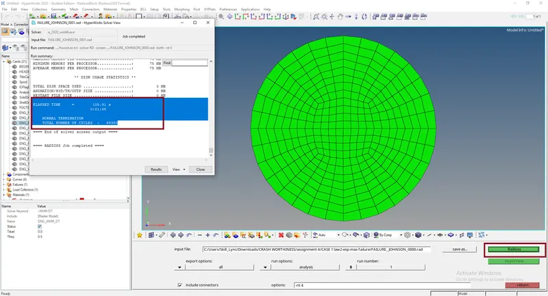
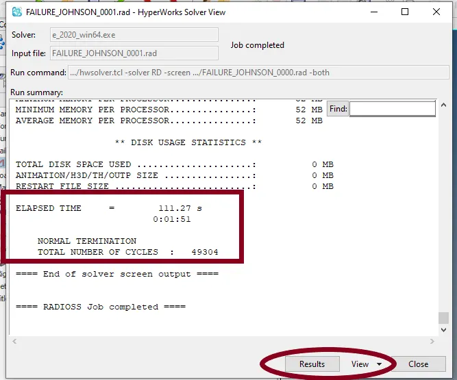
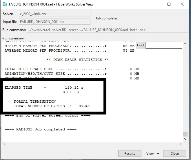
Now to run the simulation for the first case we will load the input .rad file and saving in a newfolder .to do that we go ANALYSIS-RADIOSS and click oj the input file space and load the input file from the explorer then we save it in a new folder to run the simulaton without chnging any elemet properties.after specifying the case 1 folder we will run the analysis by clicking on Radioss button .right after selecting it a popup window will come showing the runtime and simulation process that going in the solver background,after sometime it will complete the running process and gave us the info of elapsed time and number of cycles it ttok to finish the analysis .we can click on the result button wewill be redirected to HYPERVIEW.

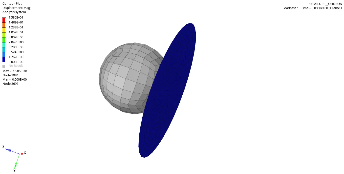
• Displacement :

• Von Mises Stress :

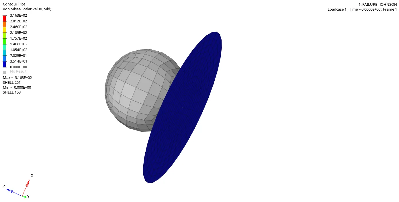
after gettting the animation of how the plate is getting deformed we have to analyze the forces and energies by plotting the graphs.to plot the graphs we will create a new window side by side and switch the mode from hyperview to hypergraph in the new window.

in hyperview we have to open .T01 file which is having all the data of simulation.after selecting the file it will ask for unit system,so we will continue the process by assigning the unit system which is already predefined to the model which can be checked in input file or under the cards tab.

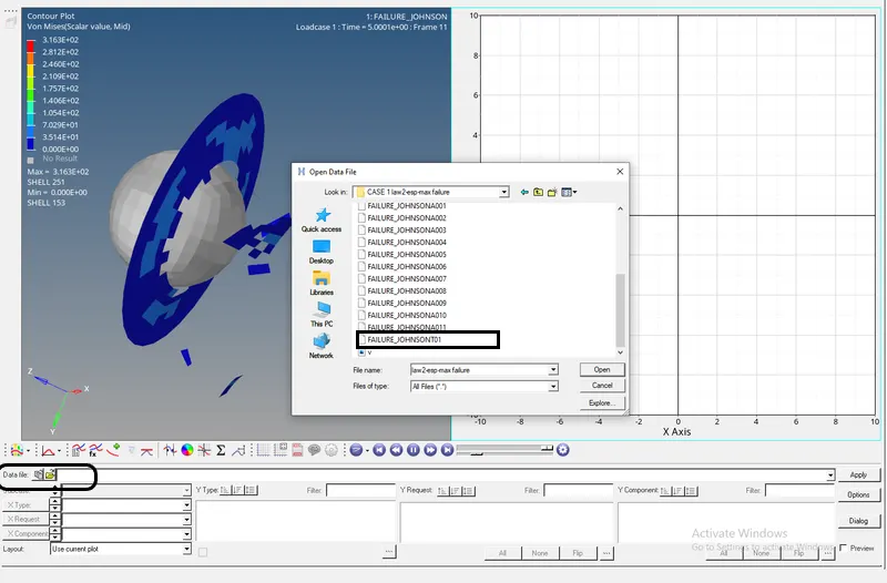
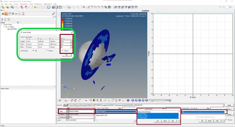
in the above image we can see that we select the global variable we need to compare i.e., internal,kinetic,horglassetc., with respect to time.

• Graph plots :

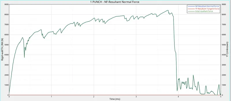
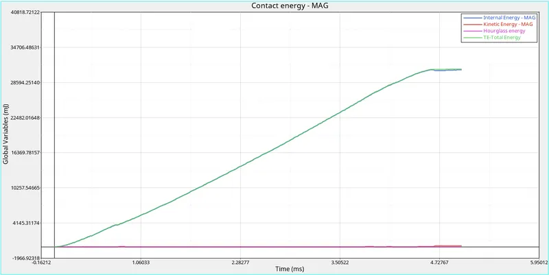
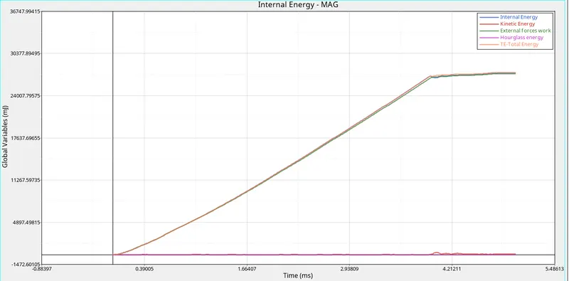
the graph below shows the plot between energies and time.

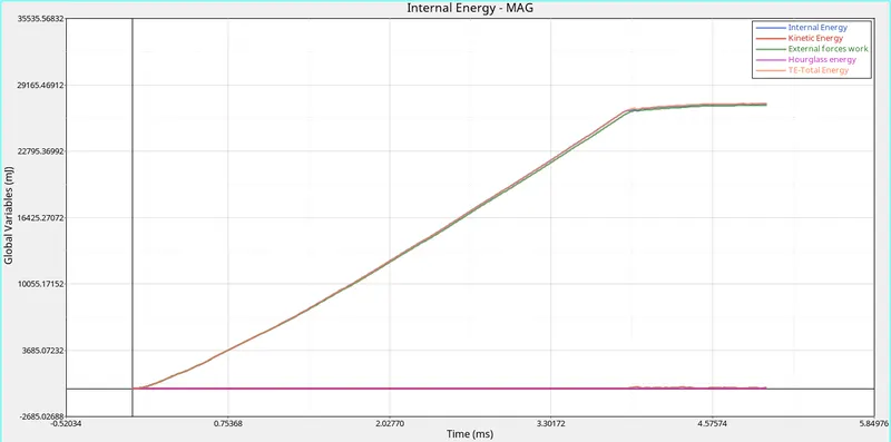
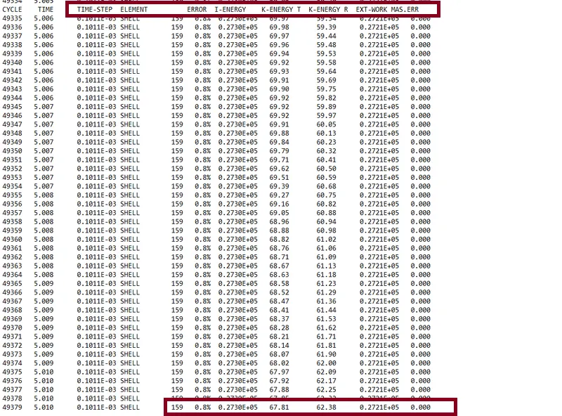
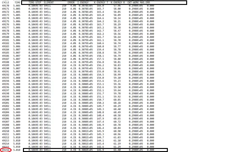
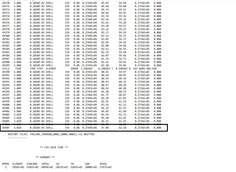
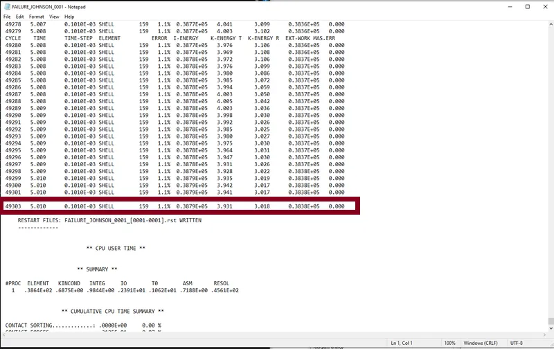
open the Radioss Engine out file in notepad and check for energy errors and mass errors present in the simulation. We find that the errors are well within the allowable range(Energy error(5 to -15%) AND Mass error(2 to 3%)) and thus the results are acceptable.

CASE 2 - LAW2_EPSMAX_CACK :

/MAT/PLAS_JOHNS/ is used as the material model

Here these values used

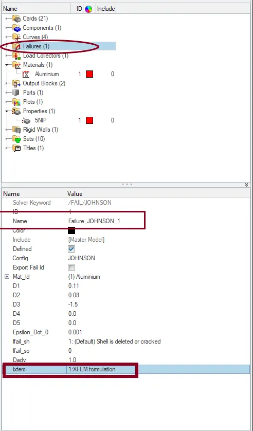
Ifail_sh = 1

Dadv = 1

Ixfem = 1, since Ixfem = 1 crack is formed when maximum plastic strain is reached in any of the integration point of an element

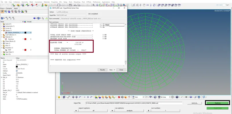
The rad file is imported in and the simulation is performed by selecting Analysis>Radioss in the bottom toolbar.

Dadv = 1 which indicates how the crack advancement will take plcae in the element. there are other values that we consider such as D1, D2, D3, D4, D5 when we change this value.The Value of D is dependent on the material and loading conditions set. So, these five values can be used to calculate the Value of D. If this value of D is greater than the Value of Dadv set, then the Crack advancement will occur according to the Dadv value. the element is deleted if a second crack is developed on it.

The next value to be changed is the value of Ixfem to 1. There are only two values in the Ixfem property, i.e 0 and 1. So if the Value of Ixfem is kept as 0, then the element will get deleted incase it fails. But, if the value of Ixfem is kept as 1, then the cracking along the meshed surfaces occurs. The Dadv value can only be used if the Ixfem is set to 1.

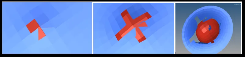
fig: propagation of crack

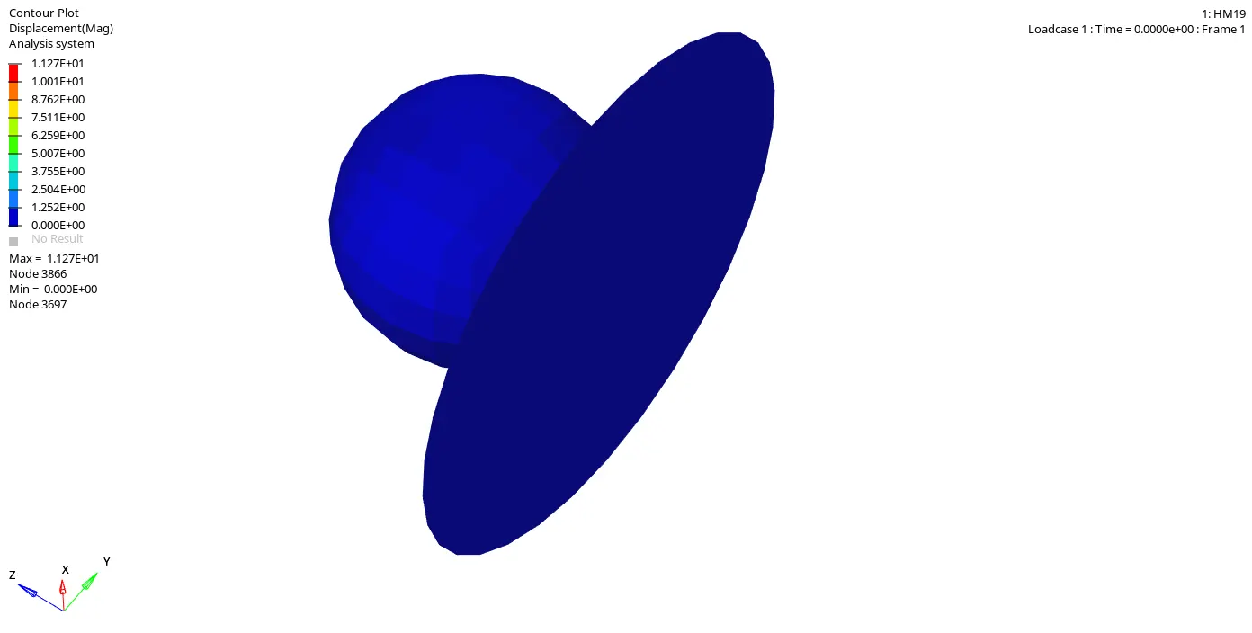
• Dispalcement

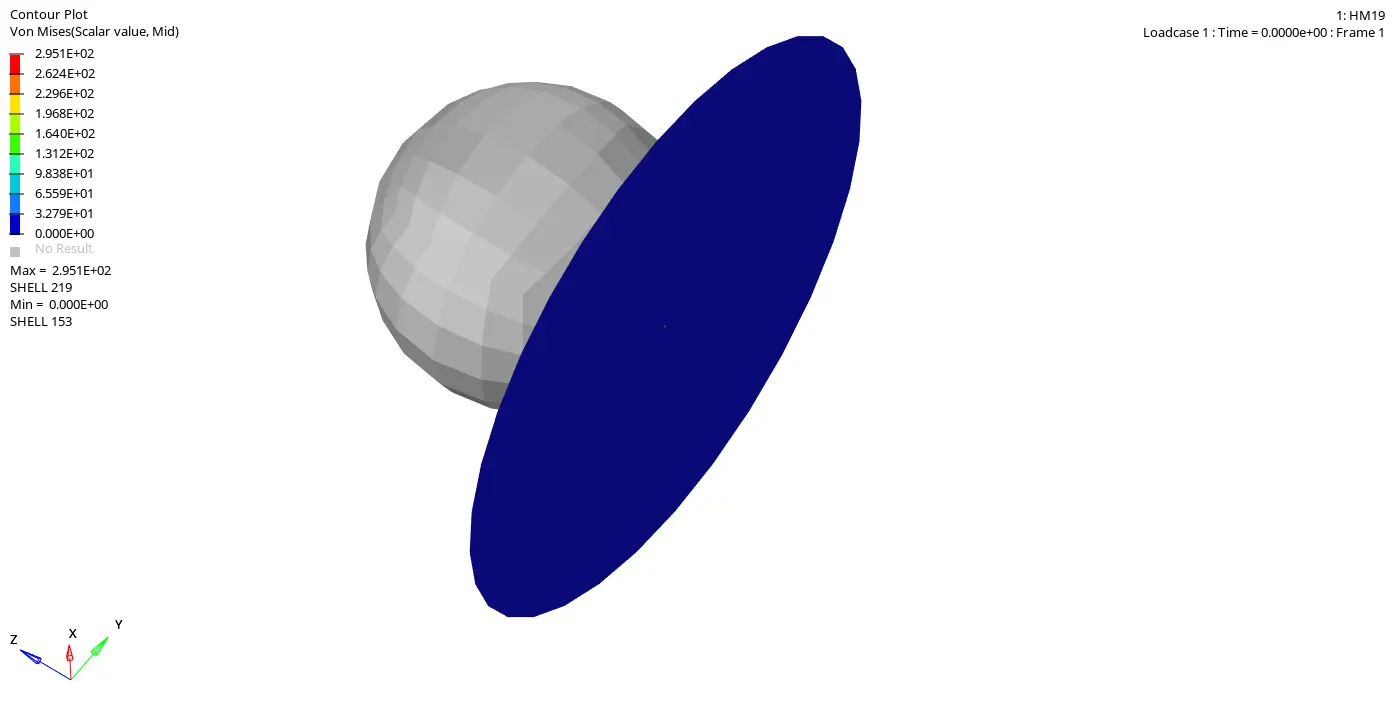
• Von Mises Stress

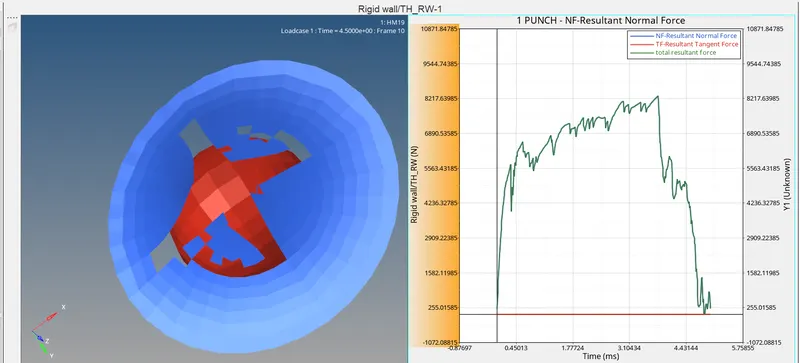
• Graph plots:

CASE 3 - Law2_epsmax_nofail :

The fail_JOHNSON card is deleted and the model is run by selecting Analysis>Radioss in the bottom toolbar.

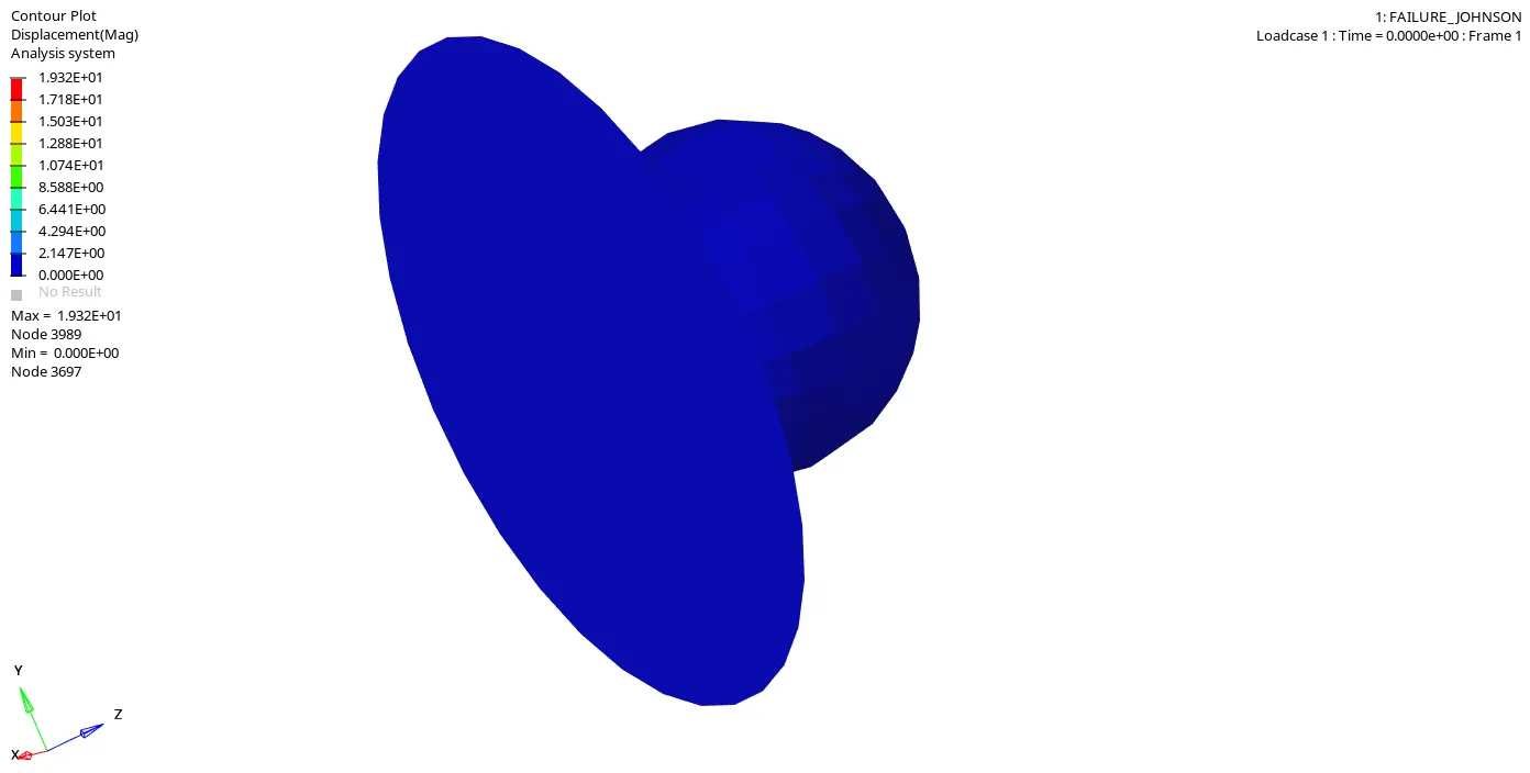
To delete this card, we simply need to right click on the failure card "Failure_JOHNSON_1" and then click on delete. Then we need to run this model and observe the graphs as well.

Displacement :

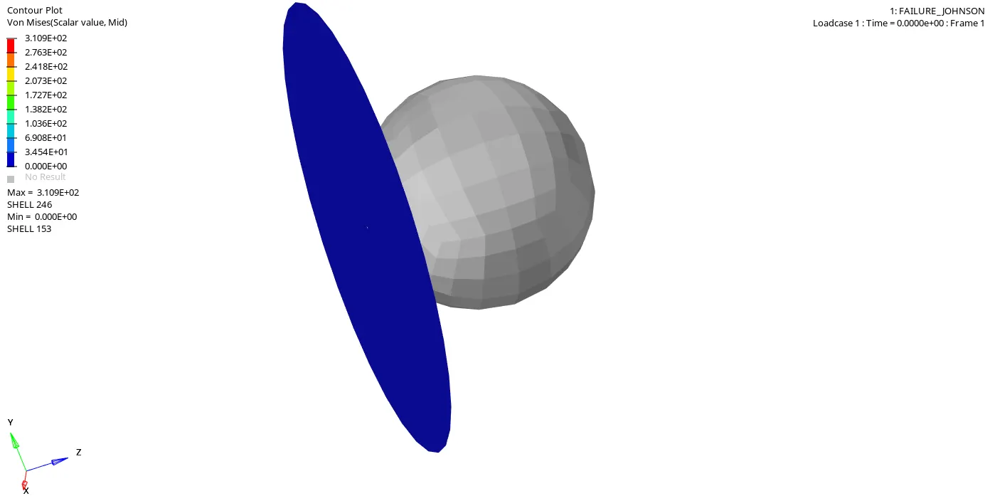
• Von Mises Stress

Graph plots:

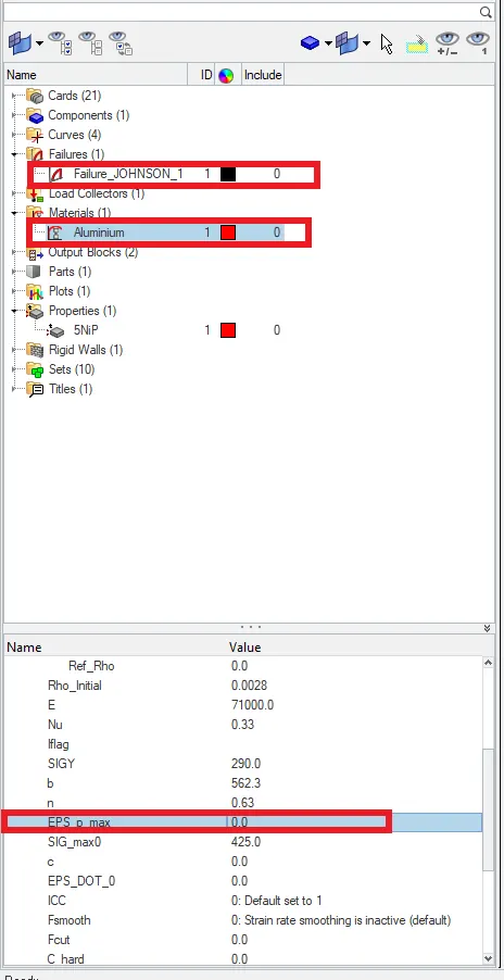
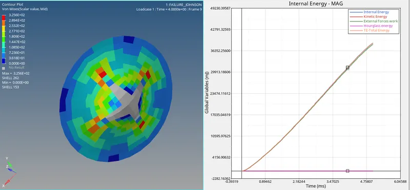
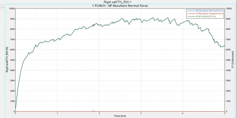
CASE 4 :Delete the EPS_p_Max and run the model with File Name Law2.

when it comes to this case we run the simulation by assigning the value for EPS_P_MAX as zero.this is what we call it the plastic strain for tension when we enter zero to it.If a higher stress is applied to the material, there will be elastic strain, but there will also be some amount of inelastic or plastic strain. This type of strain is caused by rearrangement of the atoms in the material and is not reversible. When the stress is removed the plastic deformation remains in the material.

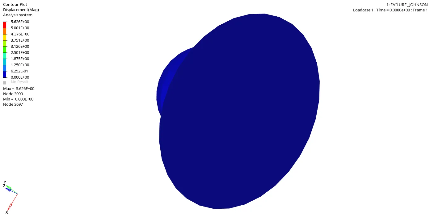
Displacement :

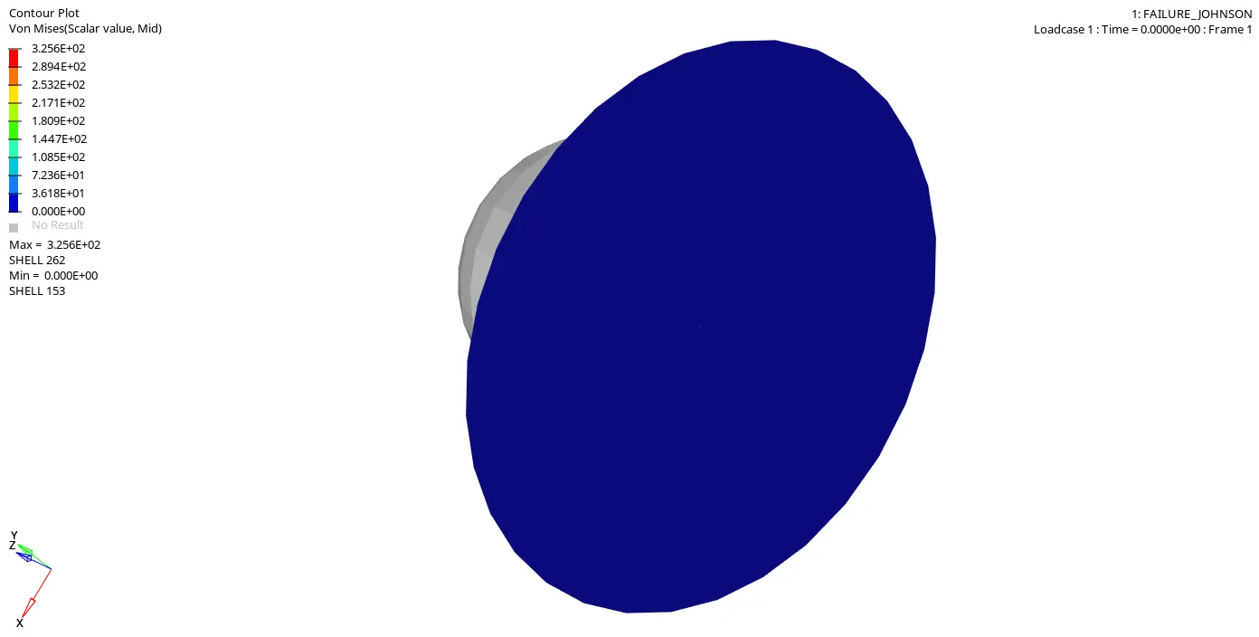
• Von Mises Stress

Graph plots:

CASE 5: Convert the material Model to Law1 Elastic with same density,E,Nu and Run.Check the results.

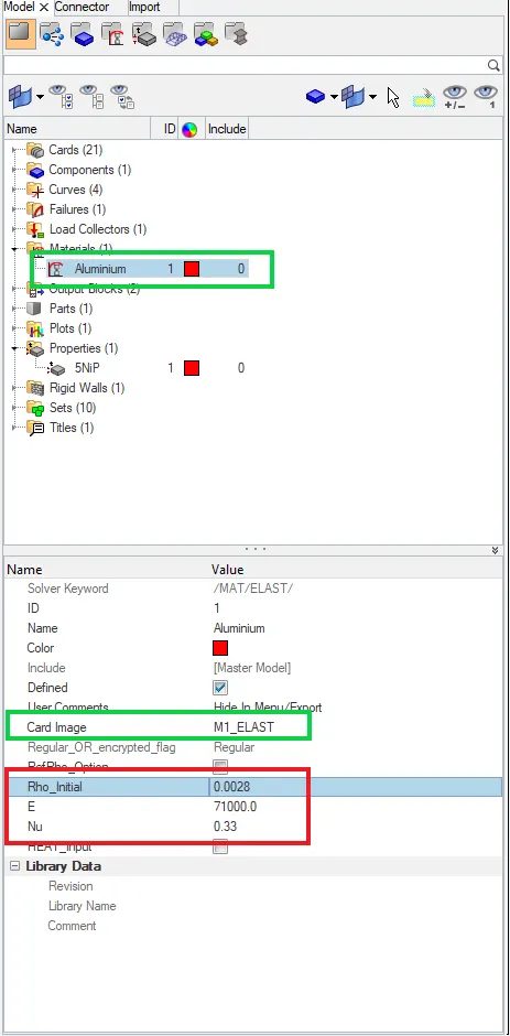
here we change the material card of the model to M1_ELAST

This law defines an isotopic, linear elastic material using Hooke's law. This law represents a linear relationship between stress and strain. It is available for truss, beam , shell and solid elements.

This material law is used to model purely elastic materials. The material stiffness is determined by only two values: the Young's modulus (E), and Poisson's ratio ( υ">υυ ). The shear modulus (G) can be computed using E and ν">ν

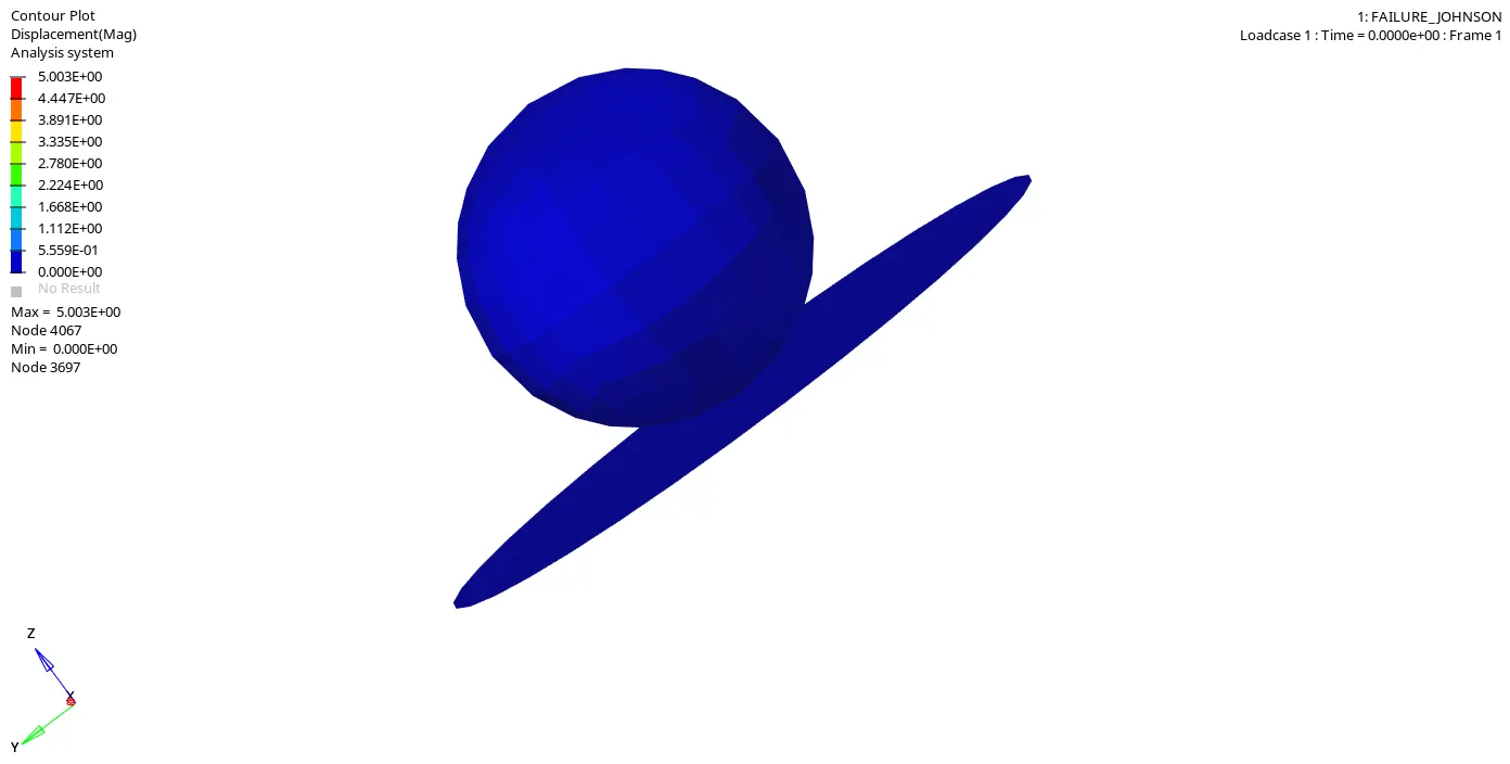
Displacement :

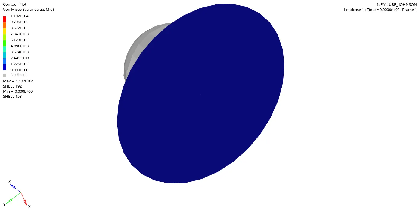
• Von Mises Stress

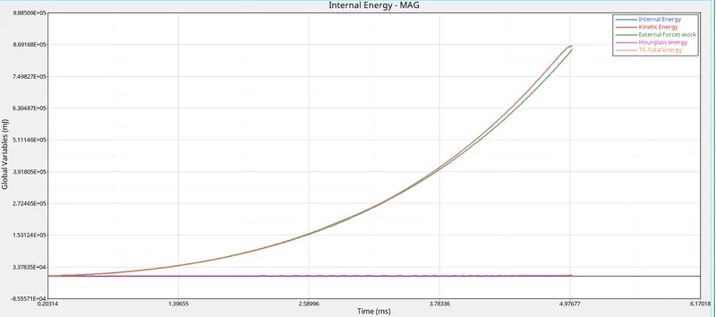
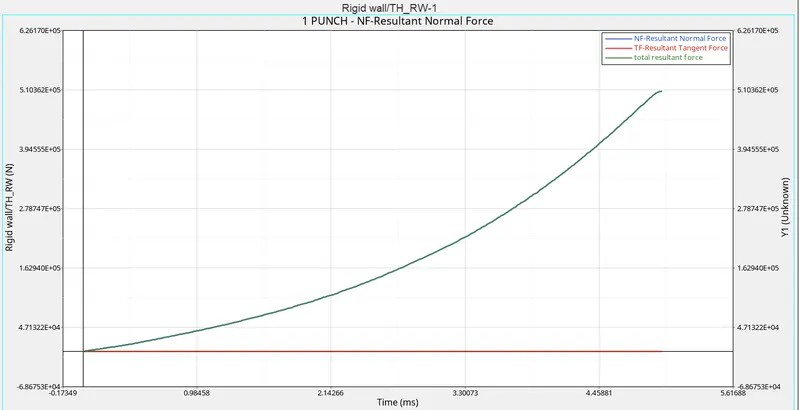
Graph plots:

CASE 6 - Law 27 :

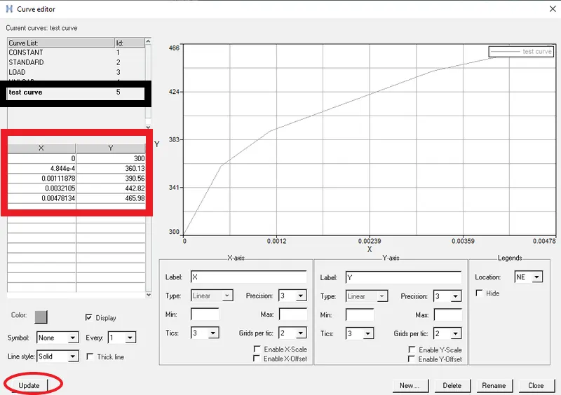
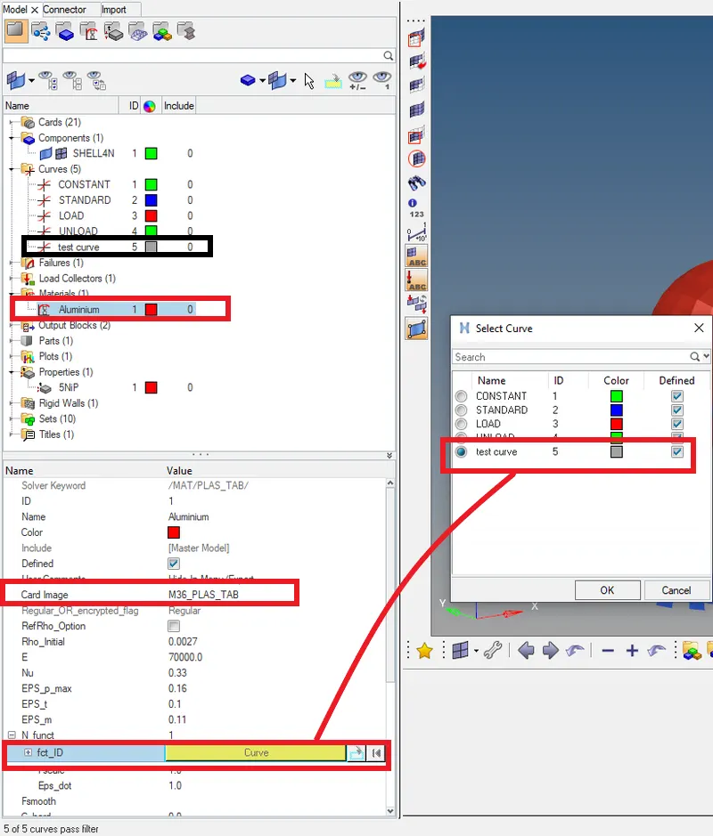
In this case we will convert the given model into Law36 i.e., Elasto-Plastic property.For the properties to be applied we will define a curve by entering the Lab Data and Create the Curve and Assign in the N Func as shown below.

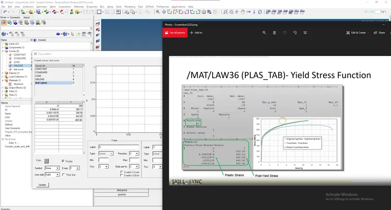
here we opened the Law1_0000.rad file.

and Created Law36 card i.e, M36_PLAS_TAB and assigned the properties as mentioned in video.

The simulation is done by selecting Radioss under Analysis option.

Once the simulation is done it give out various output files such as .RST, .ABF, .OUT, .h3d and so on.

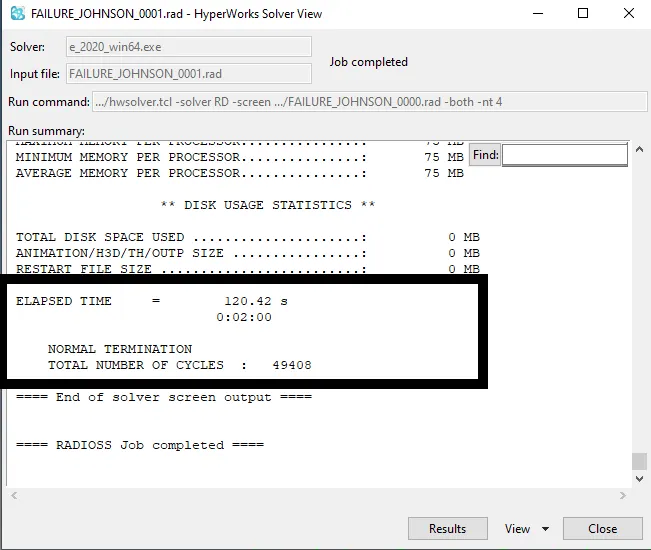
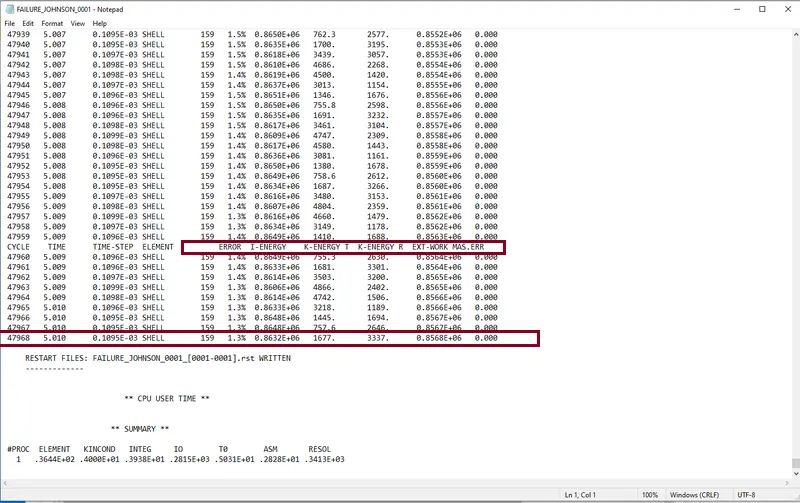
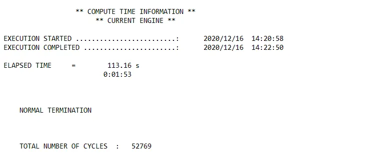
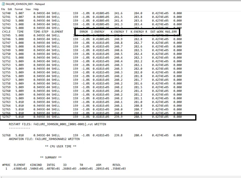
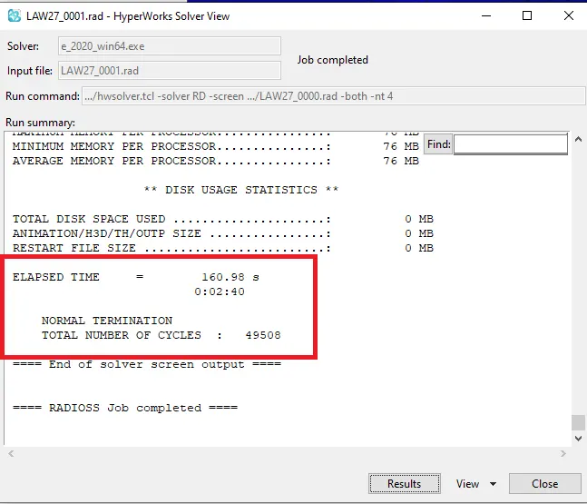
The .OUT file is used to view the no of cycles, energy error, mass error, simulation time and run time

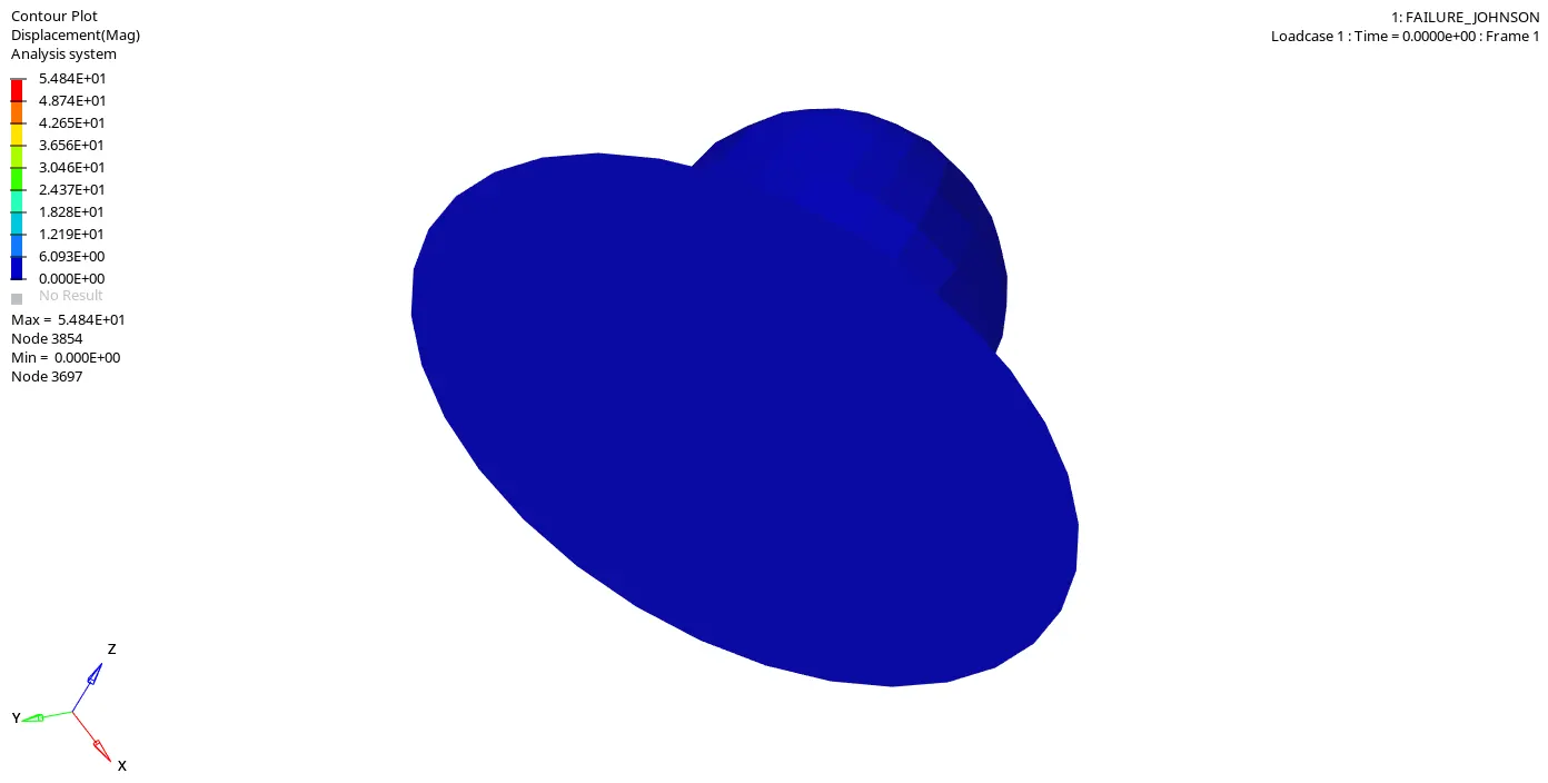
Displacement:

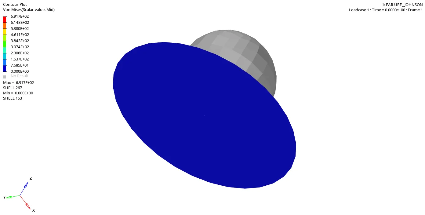
In the stress plot it is seen that even before failure occurs some elements on the outer edge are deleted, this is due to orthotropic brittle failure. It ensures the fact that in Law27 material damage is taken into account even before the failure occurs.

• Von Mises Stress

Graph plots:

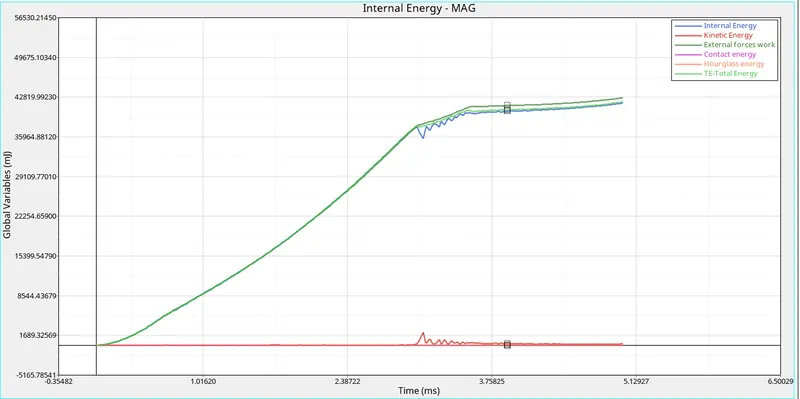
Case 6 gives total energy and internal energy curve which are almost same with minor differences, these minor differences are caused due to kinetic energy of elements of plate under impact of the Solid Sphere.

Due to usage of QEPH element formulation there is zero hourglass energy.

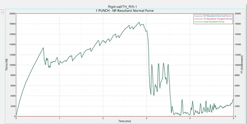
CASE 7 :

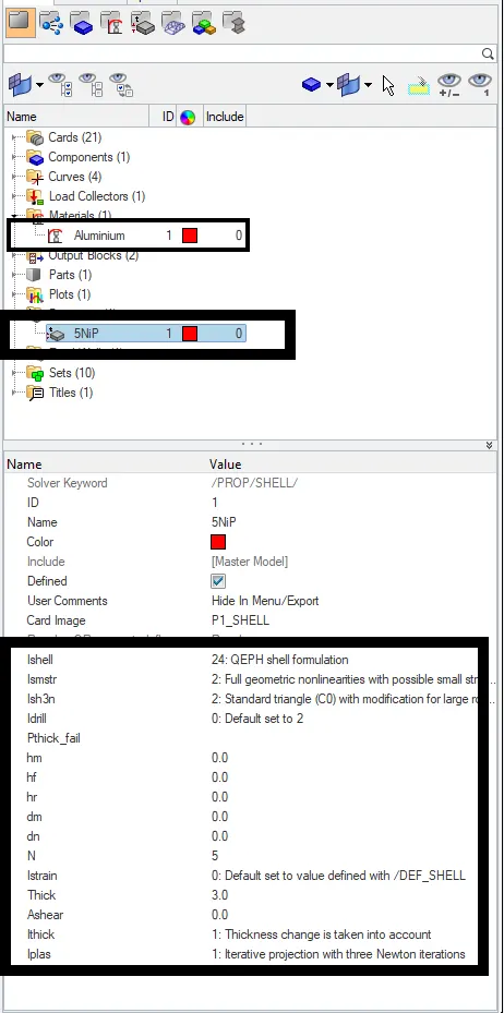
• Change the Shell properties to recomanded Properties and Notice the material properties of LAW 27

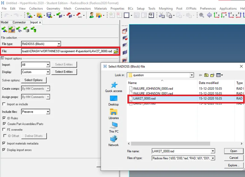
here we will import LAW27_000.rad file through selecting import solver mode button,after importing it is observed that material is assigned with LAW27 card .so we will run the simlation for this material law by assigning the recommended values to card image.

HERE ARE THE RECOMMENDED PROPERTIES WE ARE GOING TO ASSIGN TO MATERIAL CARD :

Parameters		Comment
Ishell =24		QEPH 4 nodes shells are best combination of cost and accuracy.
Ismstr=2		Full geometric non-linearities (default)with possible small strain formulation activation in RADIOSS Engine.
Ish3n=2		Standard 3 noded shell (C0)with modification for large rotation(default)
N=5		Number of integration points set to 5 for accuracy bending.
Ithick=1		Thickness change is taken into account for accuracy.
Iplas=1		Iterative plasticity for good accuracy

we go to Analysis>Select the Location to where the animated file to save .Hit on Radioss.Simulation will be carried out will be shown in the fig below:

• Dispalcement

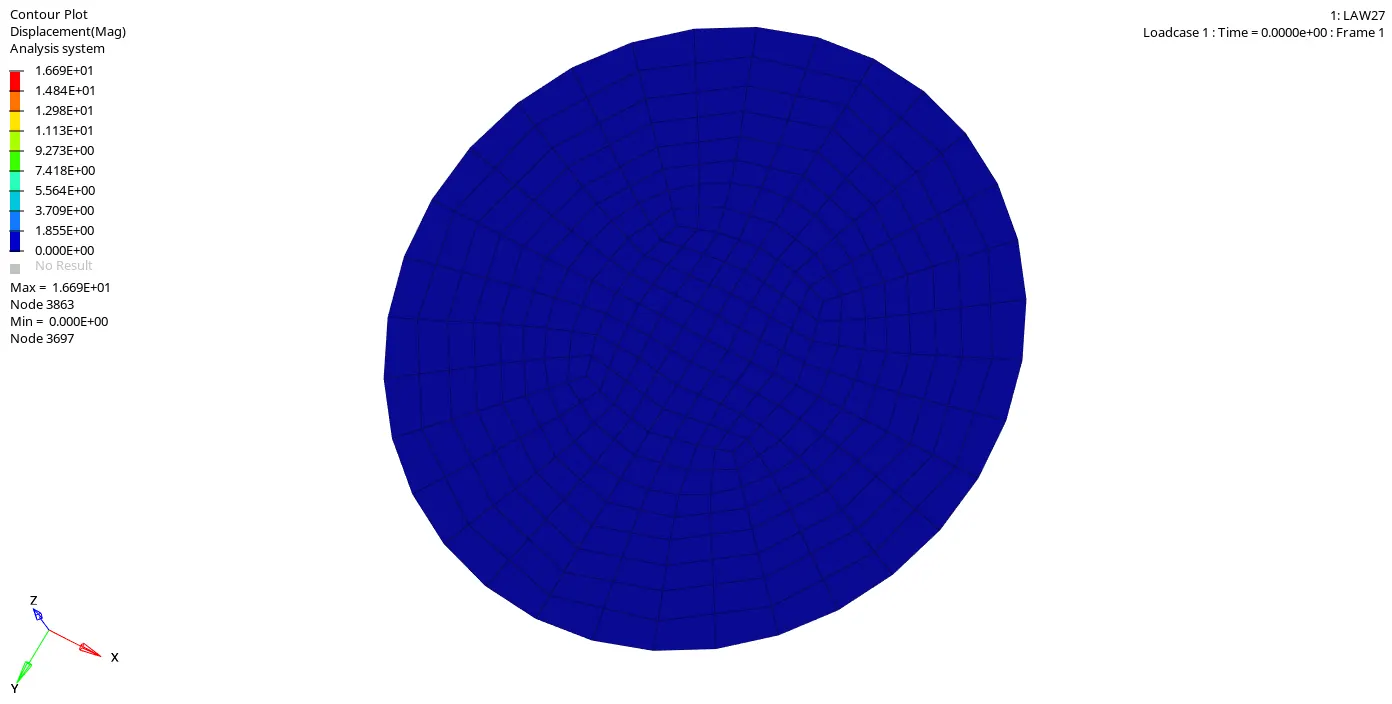
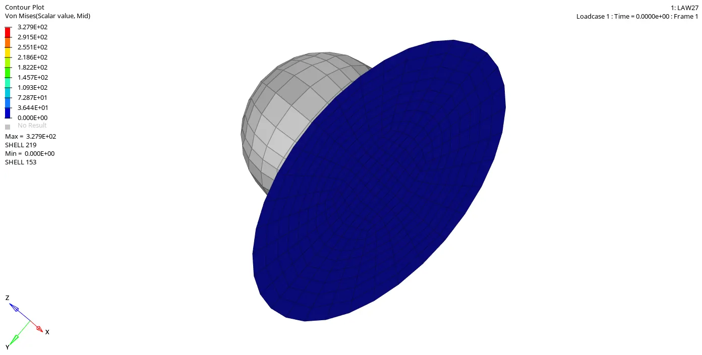
here the maximum displacement of 1.669E+01 at node 3863 and the maximum von moises stress experienced at 219th shell element location with value of 3.279+02

• Von Mises Stress

from the result of Von Misse Contour plot,Maximum Stress is 3.279E+02 and the Minimum Stress is 0.

Graph plots:

when we plotted the graph for all the energies with respect to time,it appears that hourglass energy is controlled as usually and the total and internal engergies are increasing w,r,t to time until the component reaches complete failure, after that its slightly increasing wrt to time.

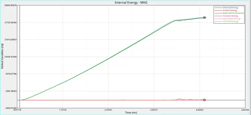
Because at initial stage we have maximum velocity, Kinetic energy is directly proportional to the Velocity. so kinetic energy is max at initial stage after hitting the KE is observed by plate so internal energy increase until the component reaches complete failure.

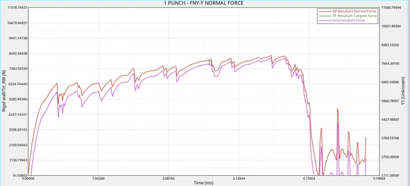
By comparing all the cases we can say that the energy errors that are obtained are very much acceptable i.e. the standard values can lie between -15 % to +5% and mass error can be seen as acceptable because it is zero.

The table which is shown below summarizes the energy error and all the other important characteristics of all the seven cases.

	NO.OF CYCLES	SIMULATION TIME (s)	ENERGY ERROR (%)	MASS ERROR (%)	MAX DISPLACEMENT (mm)	MAX VON-MOISES STRESS (GPa)
LAW2_Plas_john-Elasto plastic	49380	106.10	0.8	0	1.586E+01	3.163E+02
LAW2_Plas_john-Elasto plastic with Ixfem Formulation	49217	116.93	4.1	0	1.127E+01	2.951E+02
LAW2 without Johnson failure card	49408	120.42	0.8	0	1.932E+01	3.109E+02
LAW2 without Eps-max value(EPS-MAX=0)	49304	111.27	1.1	0	5.626E+00	3.256E+02
LAW1-M1_ELAST Elastic material (considering same values of rho,E,mu)	47969	110.12	1.3	0	5.003E+00	1.102E+04
LAW36 M36_PLAS TAB	52769	113.16	-1.0	0	5.484E+01	6.917E+02
LAW27 M27_PLAS_BRIT	49508	160.98	0.8	0	1.699E+01	3.279E+02

CONCLUSION:

As a final note we can say that this assignment helped us to understand different Material Laws used in the industry by performing this rupture plate and ball experiment with application of different material laws such as Law1, Law2, Law27 and Law36.