Rupture Plate Analysis

AIM:

To perform Analysis on Rupture Plate with different cases Given.

PROCEDURE:

CASE-1:

1. Import the solver deck Failure _jhonson_0000 file in the Hypermesh

2. Analysis is done without changing any properties and materials In It.

PROPERTY: MATERIAL:

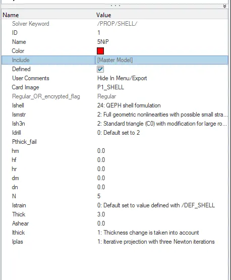
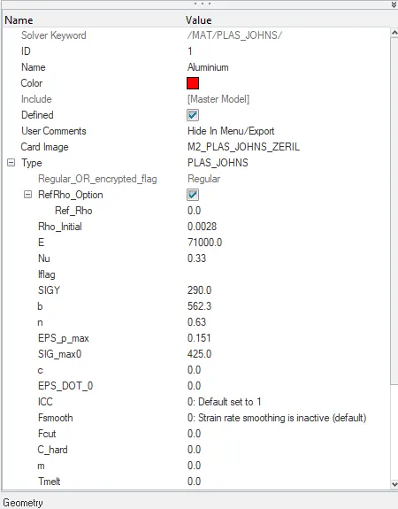
3. For Running The analysis: Analysis > Radioss is selected from the panel

4. save the radioss file as Law_2_epsmax_failiure and click Radioss.

5. The analysis runs and shows the result.

6. Click on the results from The output file to check The simulation and to find the energy and mass error.

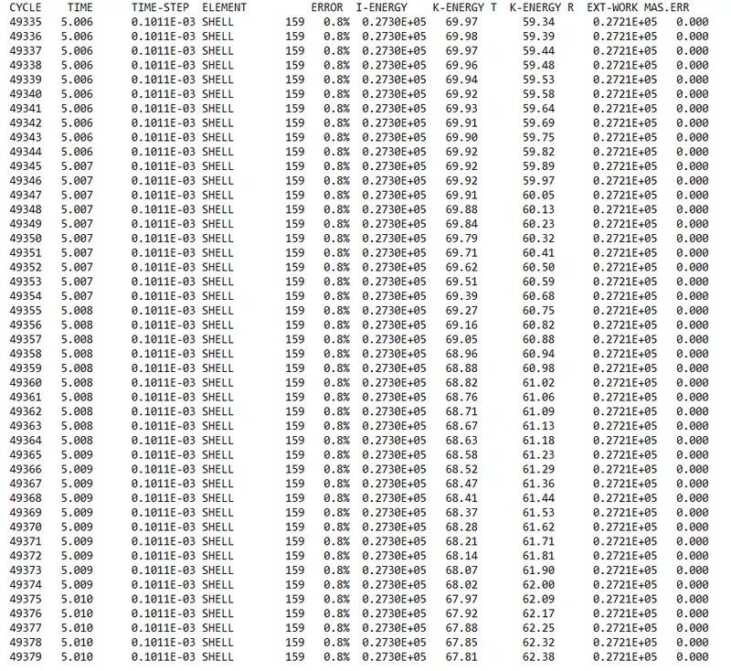
7. From the above image, the energy error is found to be 0.8% and the Mass error is found to be 0.000

8. The energy and mass error obtained is within parameters and acceptable

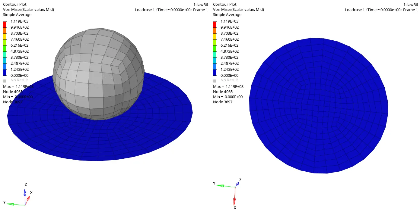
9. Click Results in the failure_0001.rad file to view in animated view and graphical view.

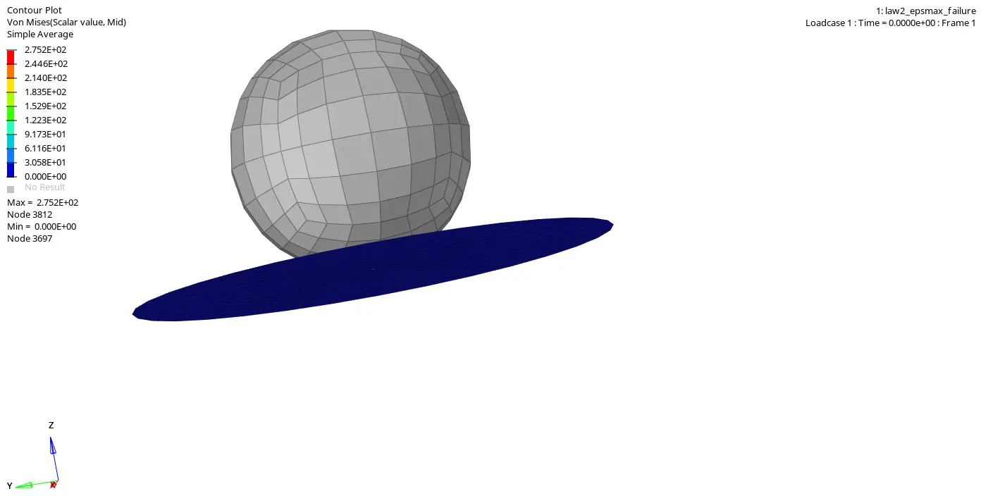
10. For the Graphical view use the Page window layout below the preferences option in Tool bar and split the screen acoording to the graph plots

11. Import T01 File from the Output file.

12. For Rigid wall, Forces choose Rigid walls > 1 punch> Total Resultant Force.

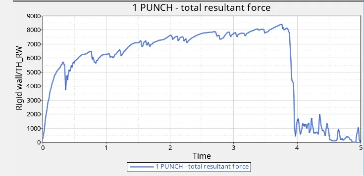
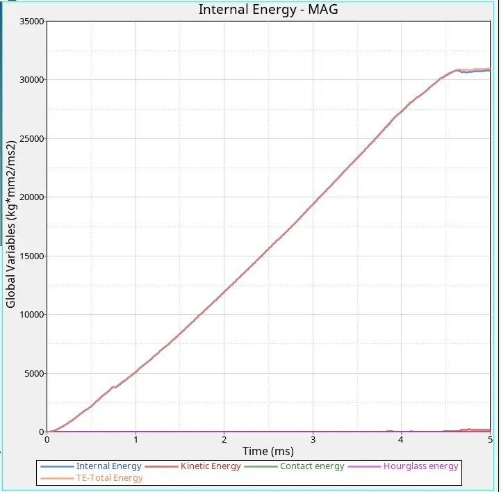
13. For the Energy graph choose the energies to be plotted, Global variables > Kinetic Energy, Internal energy, Contact energy, Hourglass energy, Total Energy > MAg and choose Apply.

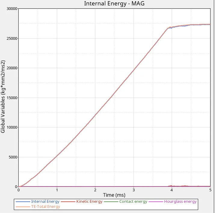
14. In the Graph, we can find the Kinetic energy shows small deflection while the Plate is breaking.

15. All the energies are summed up and shown as Total energy Which is raising linearly along

16. All the energies are initially summed up in Zero Level.

17. Hourglass energy is Found to be constant as we have used 24 QEPH formulations.

18. Contact energy is Zero in All over the process as similar to Hourglass energy.

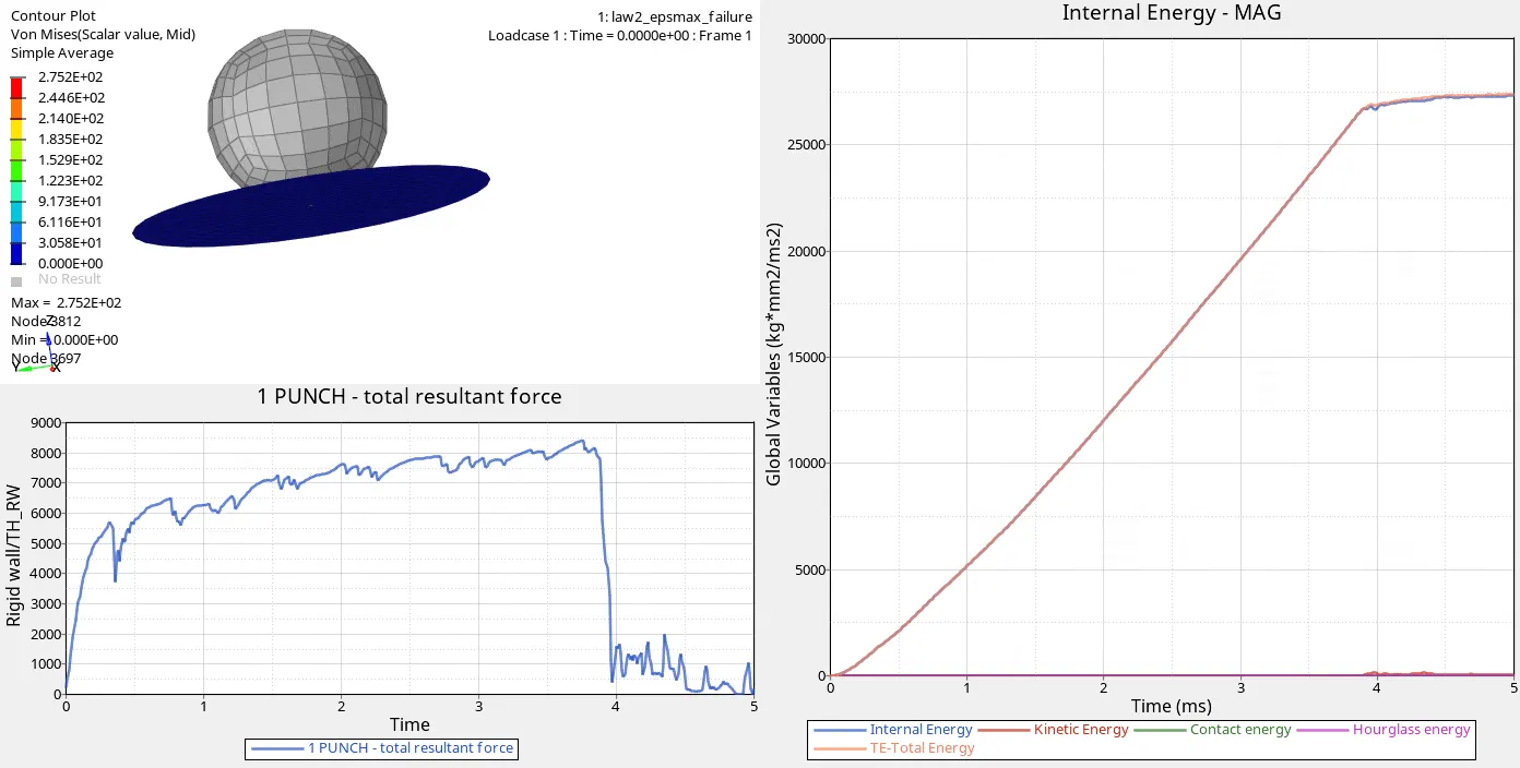
CASE:2

1. Import the solver deck Failure _jhonson_0000 file in the Hypermesh

2. The Material and property card remains unchanged as in the previous Model.

3.From The Failure card, the Boundaries are changed as given, such as Ifail_sh = 1, Dadv = 1, and IxFem = 1 (XFEM Formulation) is added to visualize the breaking down of elements.

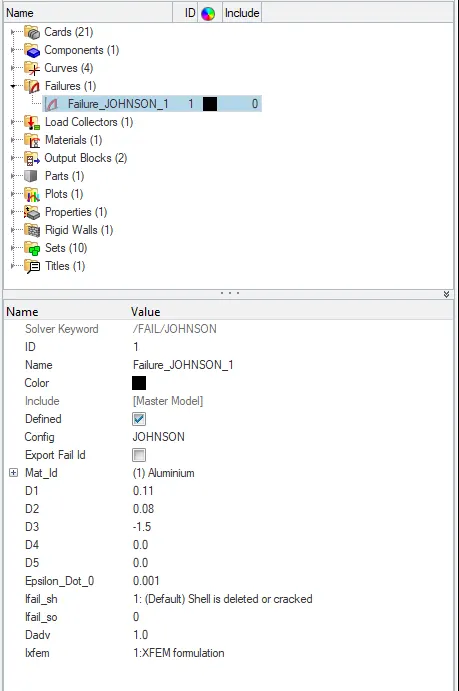
4. Save The Model as law2_epsmax_crack and run the analysis.

5. For Running The analysis: Analysis > Radioss is selected from the panel.

6.Give no of threads as -nt 4 and choose radioss.

7. The analysis Runs And Shows The Result.

8. Energy and Mass error is checked from the _0001.rad out file.

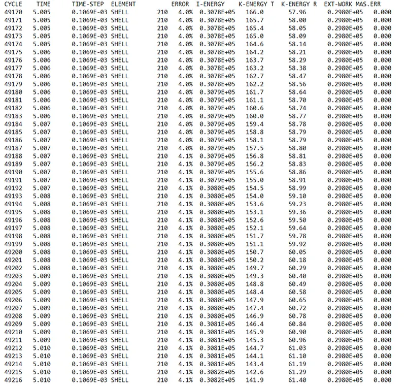
9. From the image The energy error is Found to be 4.1% and the Mass error is Found to be 0.000 which lies in the Boundary Conditions.

10. Click View Results.

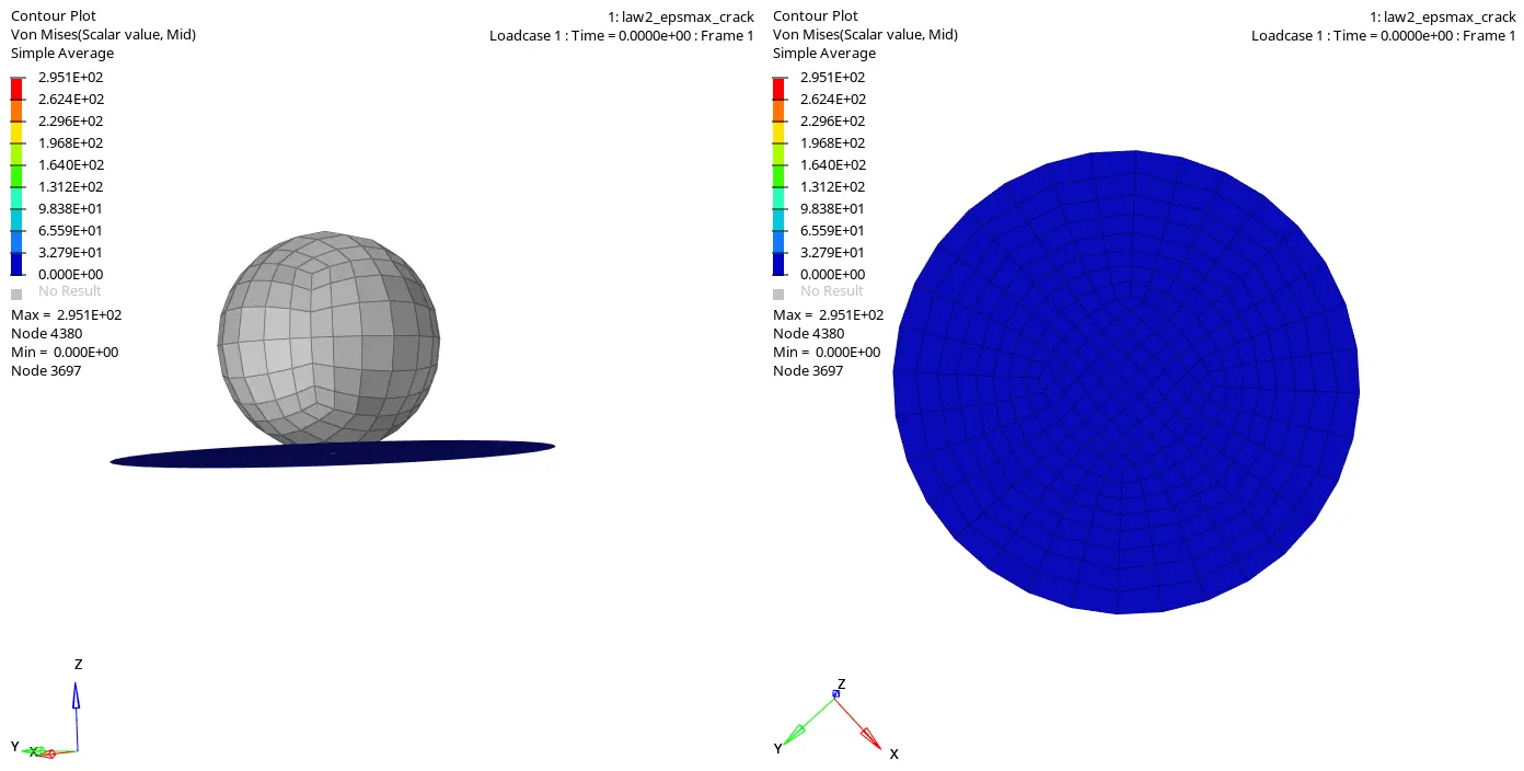
11. From The Image, We can see the crack propagation Clearly as the elements start to crack while the ball Hits and propagates to a certain distance and then breaks.

12. The IxFem =1 option is used to show the crack propagation in an optimized manner instead of element deletion.

13. As compared with the Previous model the element breaks can be analyzed in an easy manner in this.

1) without IxFem 2) With IxFEm

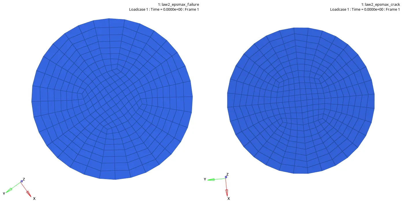
14. The analysis is similar to the previous result, but due to change in /FAIL/JOHNSON properties, we can able to find the split of elements here rather than deletion of elements due to the factors such as,

Ifail_sh (Shell failure flag) : If Ixfem =0: failure - element deleted.

If Ixfem =1: failure - element cracked.

Assigned as 1.

Dadv : Criterion for the crack advancement (Only active if with Ixfem =1).

D=∑Δ(εp/εf)≥1

Simulation of Strain Plasticity to Strain Elasticity Greater than or equal to 1,

Assigned as 1.

Ixfem = 0 (Default) Without XFEM

XFEM formulation= 1

15. For the Graphical view use the Page window layout below the preferences option in Tool bar and split the screen acoording to the graph plots

16. Import T01 File from the Output file.

17. For Rigid wall, Forces choose Rigid walls > 1 punch> Total Resultant Force.

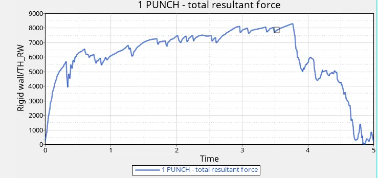
18. For the Energy graph choose the energies to be plotted, Global variables > Kinetic Energy, Internal energy, Contact energy, Hourglass energy, Total Energy > MAg, and choose to Apply.

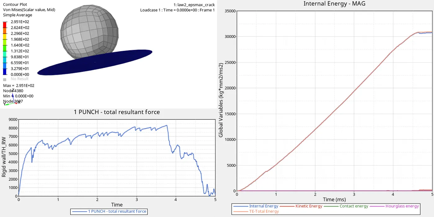
CASE 3:Law 2 without /Fail/Johnson.

1. Import the solver deck Failure _jhonson_0000 file in the Hypermesh

2. The Material and property card remains unchanged as in the previous Model.

3. The failure model card "/Fail/Johnson" is removed to observe any change in results.

4.Right click on The Failures and choose delete.

5. For Running The analysis: Analysis > Radioss is selected from the panel

6. save the radioss file as Law_2_epsmax_nofail and click Radioss.

7.Give no of threads as -nt 4 and choose radioss.

8. The analysis Runs And Shows The Result.

9. The energy and The Mass errors are checked from the OUT file.

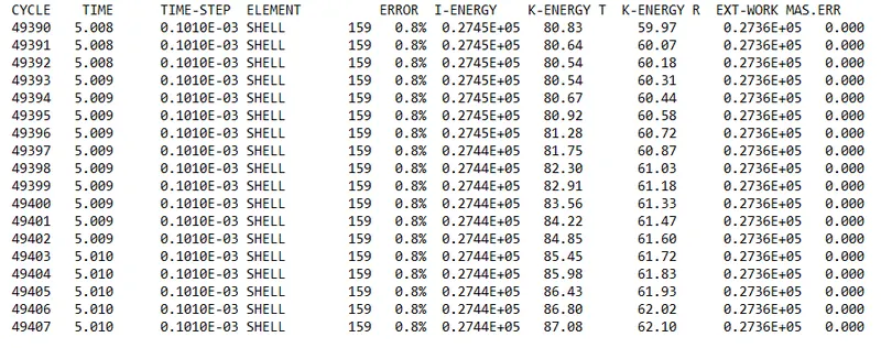
7. From the image, we can find that the Energy error is 0.8% and Mass error is 0.000 which lies in the conditions.

8. Click on results to view animation and graphical files.

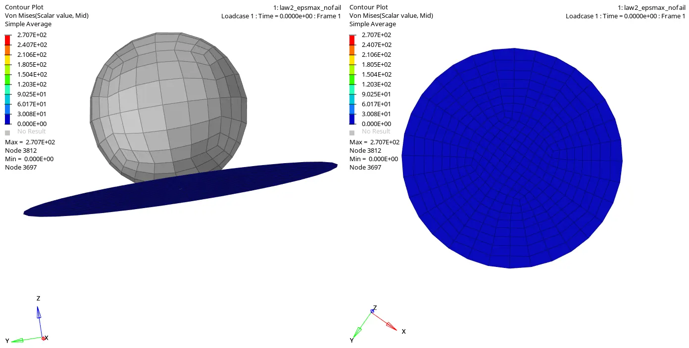
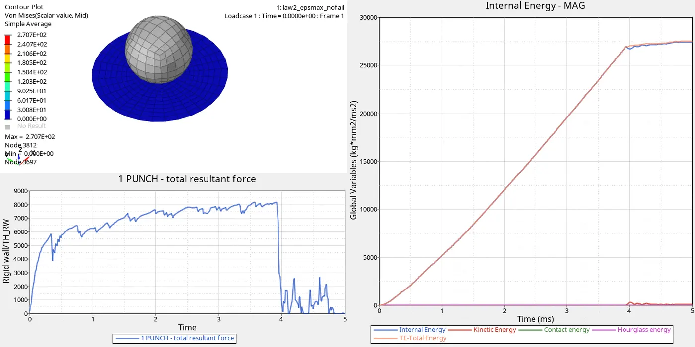
9. From the above image, we can find that the elements getting deleted while the ball impacts on the plate whereas in the previous component the elements getting Cracked can be viewed.

10. For the Graphical view use the Page window layout below the preferences option in Tool bar and split the screen acoording to the graph plots

11. Import T01 File from the Output file.

12. For Rigid wall, Forces choose Rigid walls > 1 punch> Total Resultant Force.

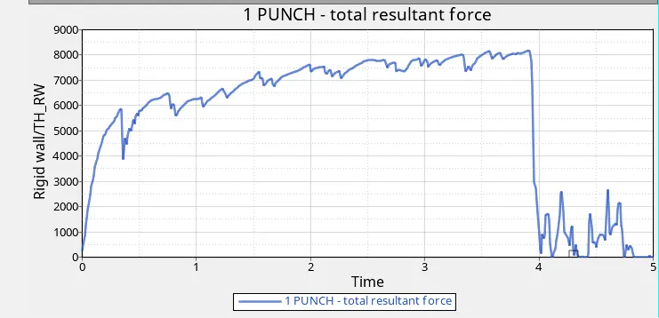
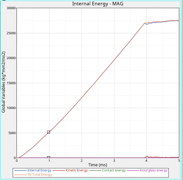
13. For the Energy graph choose the energies to be plotted, Global variables > Kinetic Energy, Internal energy, Contact energy, Hourglass energy, Total Energy > MAg, and choose to Apply.

INTERFACE:

• The internal energy shows the work done on the element in which it is a deformation of the plate.
• As the failure formulation is deleted here, instead of elemental cracking, the elements gets deleted.
• Hourglass is not observed.
• Contact Energy is Zero.

CASE 4: Law 2 with EPS_p_max value infinite.

1. Import the solver deck Failure _jhonson_0000 file in the Hypermesh.

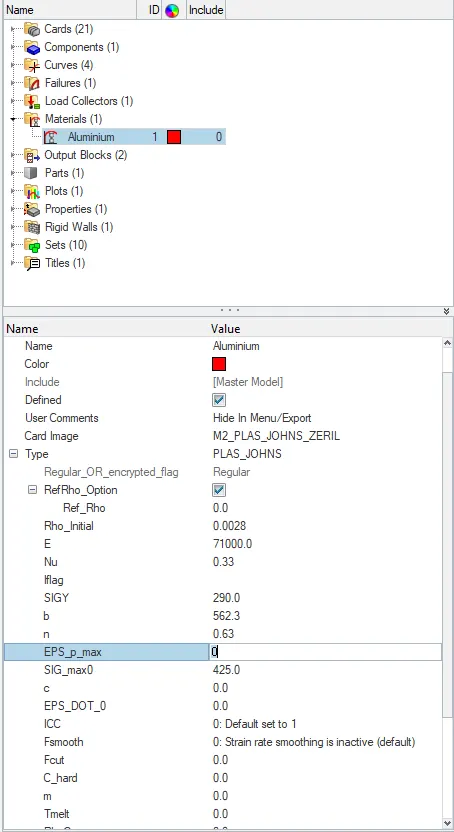
2.From the material Card change the value of Eps_p_max value as 0

3.The Eps_p_max value refers to the maximum permitted plastic strain

4.For Running The analysis: Analysis > Radioss is selected from the panel

5. save the radioss file as Law_2 and click Radioss.

6.Give no of threads as -nt 4 and choose radioss.

7. The analysis Runs And Shows The Result.

8. The energy and The Mass errors are checked from the OUT file.

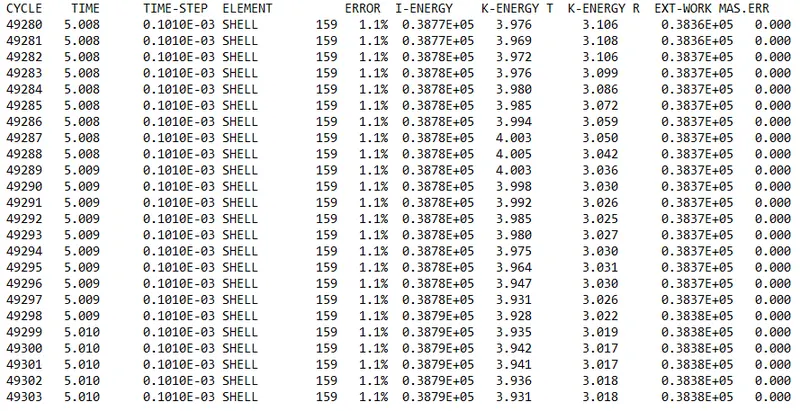
9. From The Image the Energy error is 1.1% and the mass error is 0.000 lies within the boundary Conditions.

10. Click on results to view in graphical and animated mode.

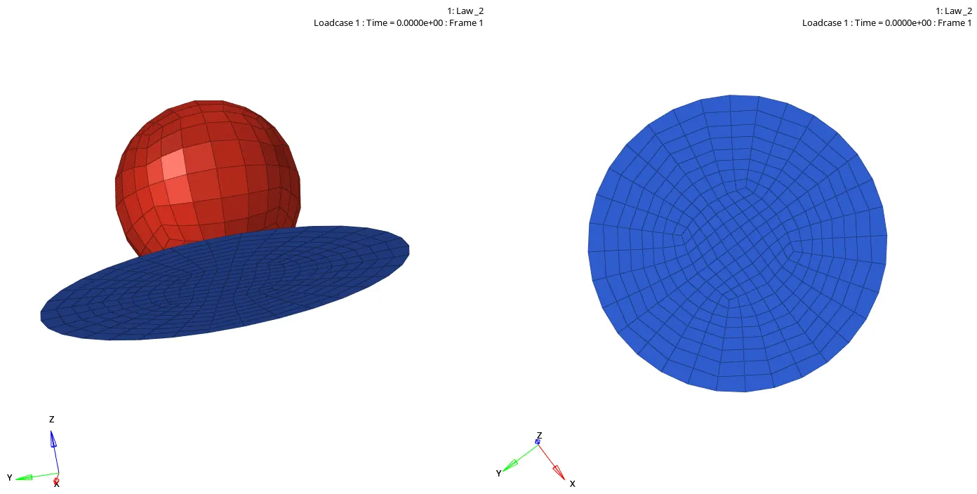
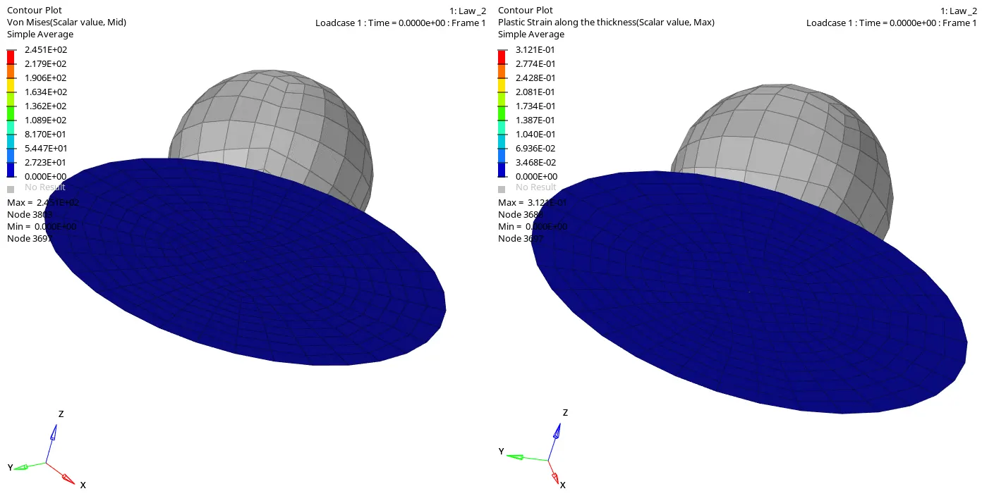
11. As the Eps_p_max value is assigned to 0 the element will not fail as it was like an inbuilt failure card for the plastic Components so there won't be any failure like before.

(As in this model Since the failure card is assigned the component tends to break, if the failure card is deleted it behaves like elastic in form.)

12.For the Graphical view use the Page window layout below the preferences option in Toolbar and split the screen according to the graph plots

13. Import T01 File from the Output file.

14. For Rigid wall, Forces choose Rigid walls > 1 punch> Total Resultant Force

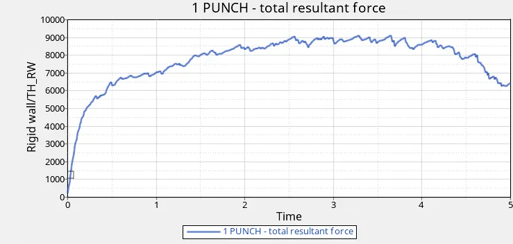
15.For the Energy graph choose the energies to be plotted, Global variables > Kinetic Energy, Internal energy, Contact energy, Hourglass energy, Total Energy > MAg, and choose to Apply.

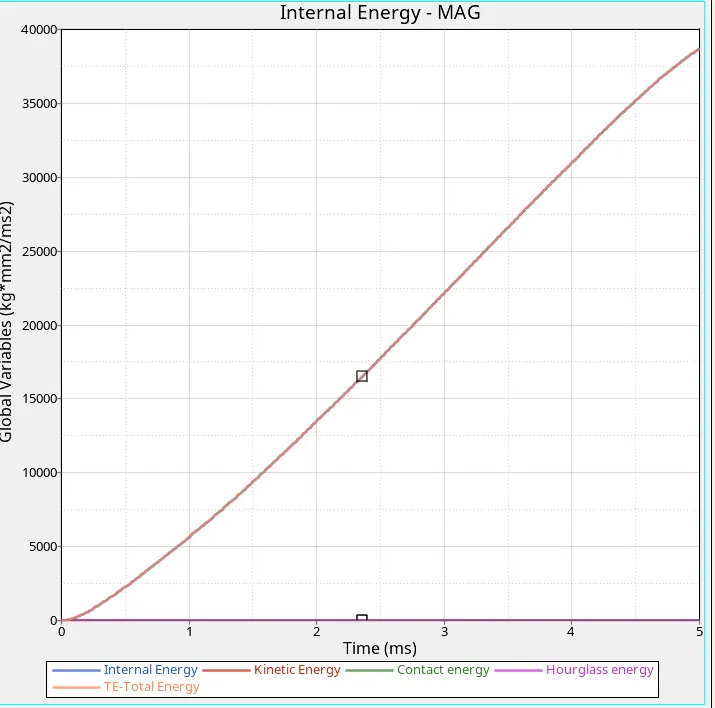
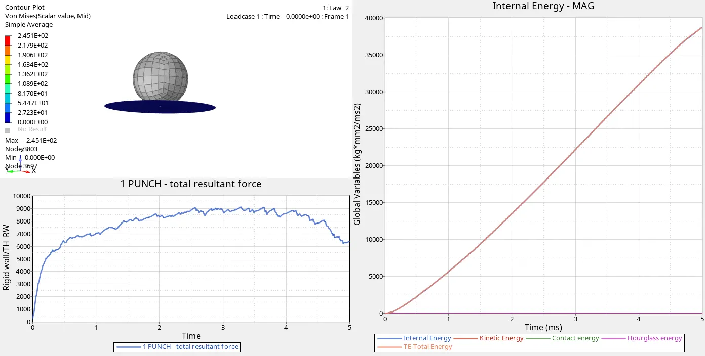
16.Internal energy increases linearly, in which the total energy sums up, stably over IE.

17. There is no involvement of hourglass energy, contact energy, and kinetic energy in the aluminum component.

CASE 5: Law 1 elastic material

1. Import the solver deck Failure _jhonson_0000 file in the Hypermesh.

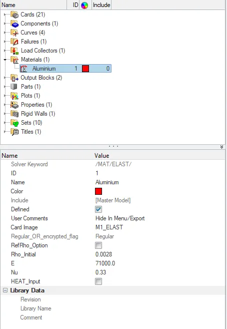
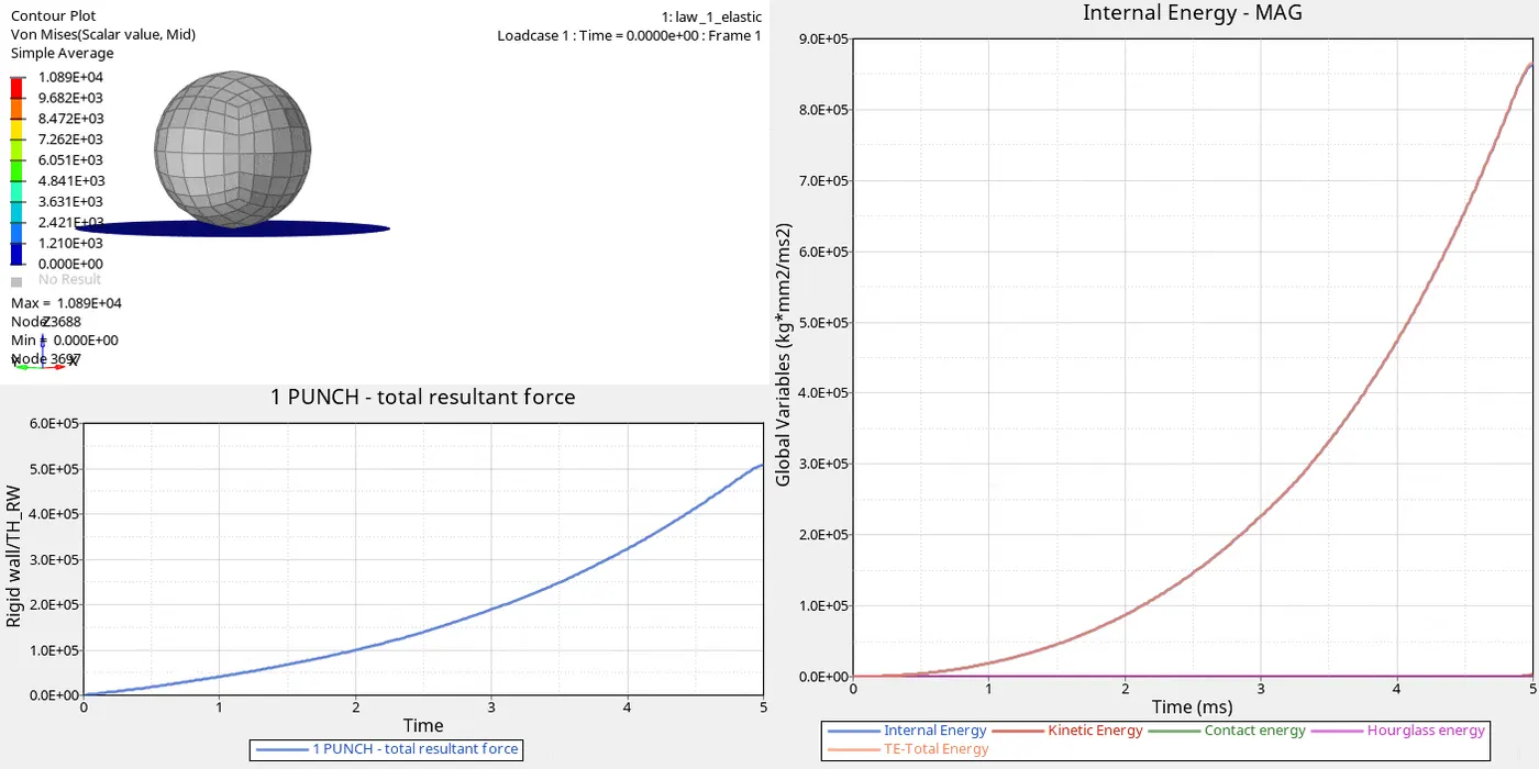
2. In this case, the whole material card is changed to M1_ELAST so the material will behave like an ideal elastic material that follows Hooke's law up to the elastic limit.

3.The basic E, Rho, and Nu values are given as the inputs to proceed with the analysis.

4. The values are taken from The Videos.

5. Now click on the analysis panel in the hypermesh.

6.Select Radioss option the save the model in a local directory.

7.Click the Radioss to run the simulation.

8.Save the Model As Law 1 elastic.

9. The analysis Runs And Shows The Result.

10. The energy and The Mass errors are checked from the OUT file.

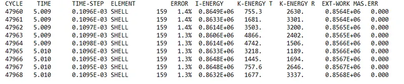
as the energy error is 1.3% which is less than 15% so it is acceptable, also the mass error is found out to be 0.000

11.Click on The results to view them in animated format.

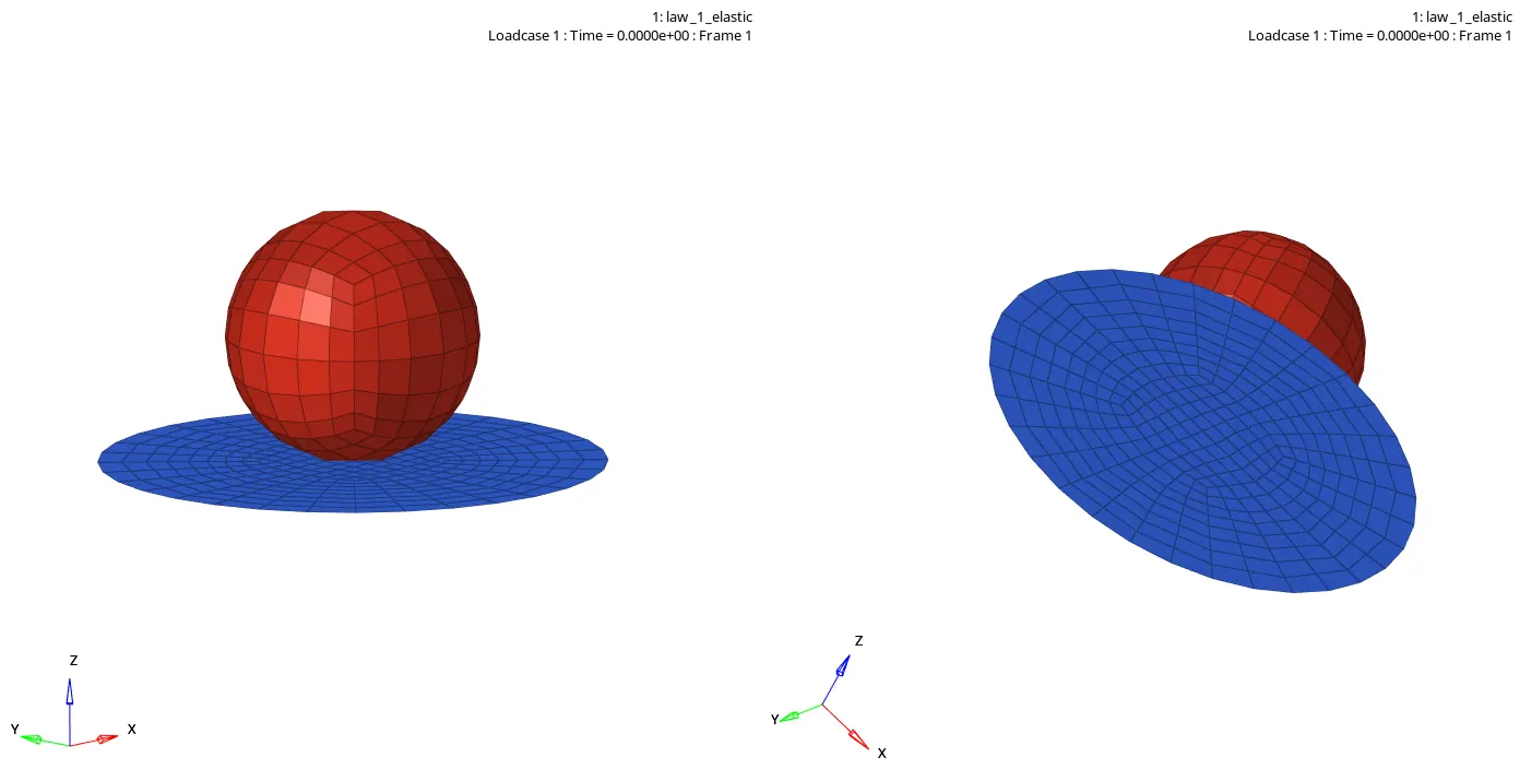
12.Apply voinmises data over it to view solver analyzed stress and strain acting on It.

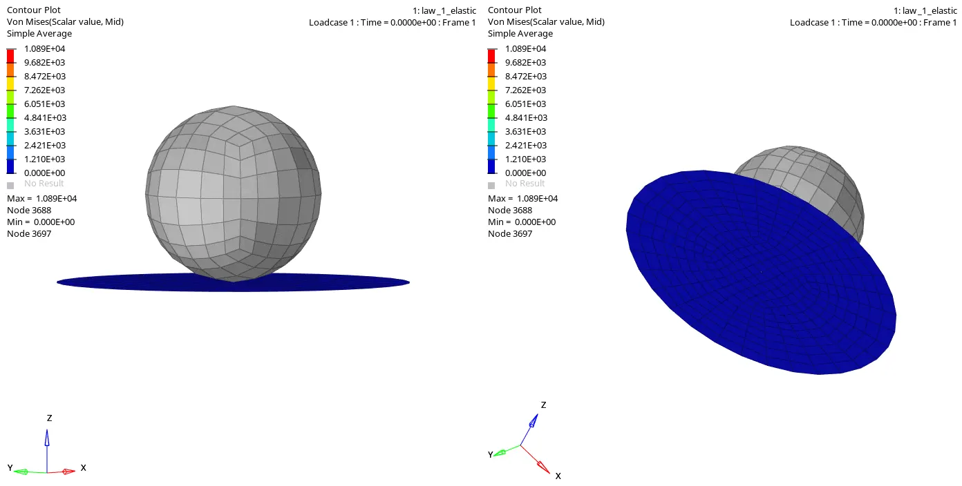
13. since the elastic material is applied the component shows elastic behavior instead of elements getting cracked or deleted.

14. It applies for linear elastic material Based on Hooke's law.

15.Theis material card is used purely for Plastic materials.

16.For the Graphical view use the Page window layout below the preferences option in Toolbar and split the screen according to the graph plots

17. Import T01 File from the Output file.

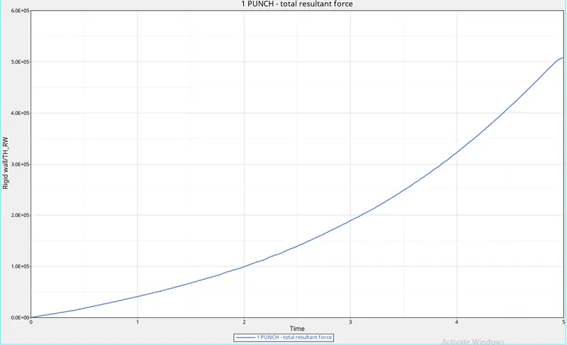
18. For Rigid wall, Forces choose Rigid walls > 1 punch> Total Resultant Force

19.For the Energy graph choose the energies to be plotted, Global variables > Kinetic Energy, Internal energy, Contact energy, Hourglass energy, Total Energy > MAg, and choose to Apply.

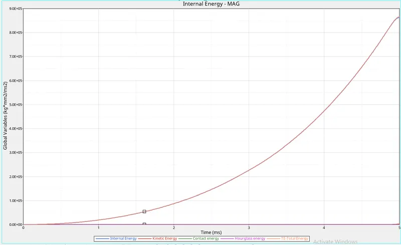
20.There is No contact energy & Hour glass energy observed.

21.The curve is found to be smooth based on the resultant force of the rigid ball, which is an area of elasticity.

22.The total energy is constant throughout the process, as the mass error is found to be zero.

Case 6: Law 27 PLAS_BRIT material

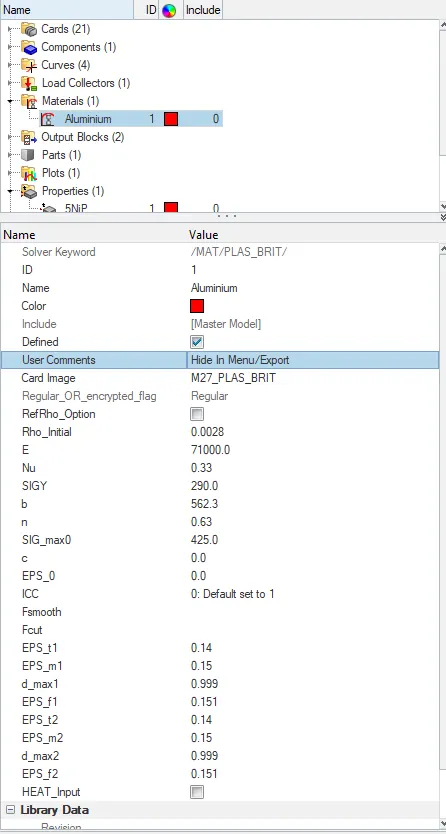
This law is known as isotropic elastoplastic Johnson-Cook material model with an orthotropic brittle failure Properties

1. Import the solver deck LAW27_0000.rad file in the Hypermesh.

2.Check for The Material and Properties and edit if needed.

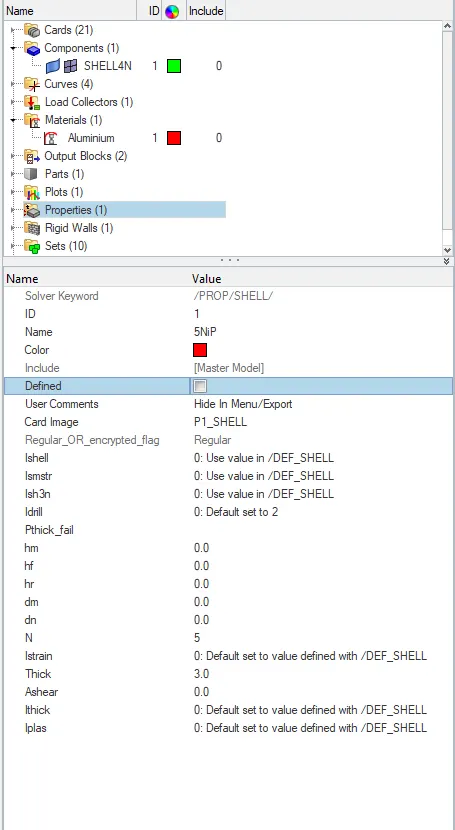
MATERIAL PROPERTIES

3. Now click on the analysis panel in the hypermesh.

4. Select Radioss option the save the model in a local directory as Law_27.

5. Click the Radioss to run the simulation.

6. The analysis Runs And Shows The Result.

7. The energy and The Mass errors are checked from the OUT file.

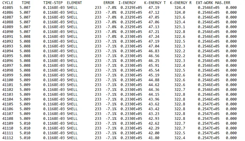
8.as the energy error is -7.1%, also the mass error is found out to be 0.000.

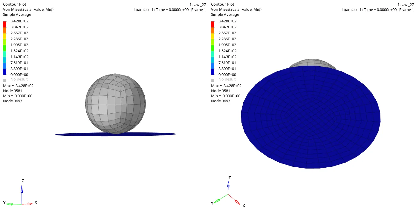
9.Click on The results to view them in animated format.

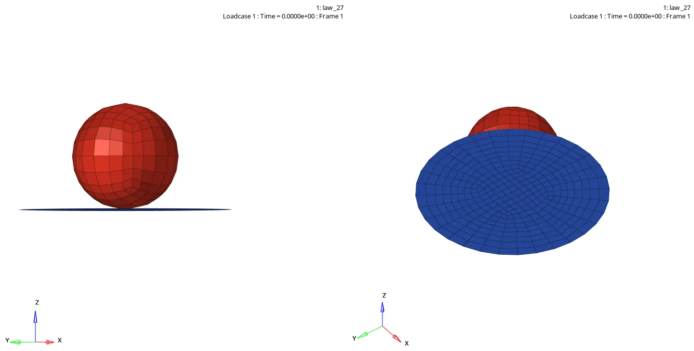
10.Law 27 is elastic brittle Material.

11. As we can see The Element is Getting Deleted.

12.The Element when it Reaches the max strain value it breaks down Abruptly eg breaking glass.

13.For the Graphical view use the Page window layout below the preferences option in Toolbar and split the screen according to the graph plots

14. Import T01 File from the Output file.

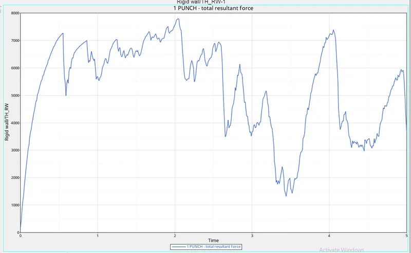
15. For Rigid wall, Forces choose Rigid walls > 1 punch> Total Resultant Force

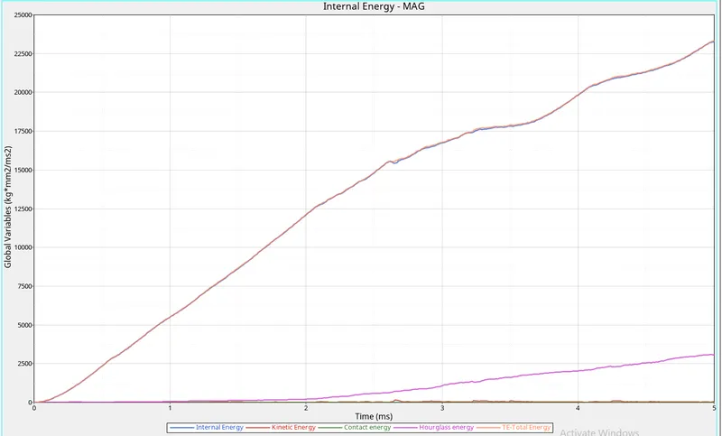
16. For the Energy graph choose the energies to be plotted, Global variables > Kinetic Energy, Internal energy, Contact energy, Hourglass energy, Total Energy > MAg, and choose to Apply.

17.The Resultant forces show the ball striking the aluminum component and rupturing it.

18. Hourglass energy is produced when deformation occurs in the component.

19.Internal energy shows the deformation takes place as work is done.

20.Kinetic energy is very low during the process.

21.The total energy is a bit unstable as there is a considerable amount of hourglass energy acting on the component.

CASE:7Law 36 PLAS_TAB Material

1. Import the solver deck Failure _jhonson_0000 file in the Hypermesh.

2.Change the MAterial card to M36_Plast_TAb by Material >Aluminium > Properties > Change card image to M36_PLAS_TAB.

3.Assign The parameters for The Materials As given in The slides.

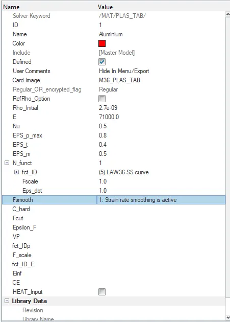
4.Change The N function to 1 to plot The graph

5.For Plotting The Graph Right Click On the curves and Choose to Create.

6.create New Curve and Assign The values Given In the Slides or Data and Choose Update.

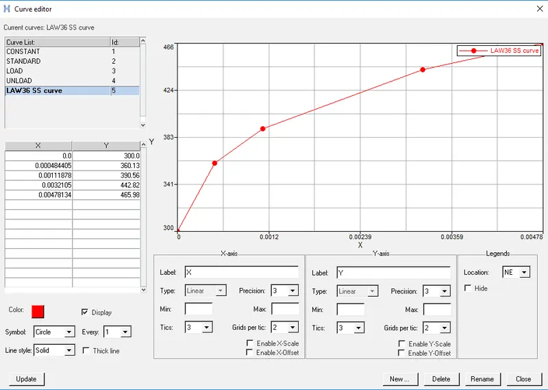
7.Update the Curve in the material to Run The Simulation.

8.Now click on the analysis panel in the hypermesh.

9. Select Radioss option the save the model in a local directory as Law_27.

10. Click the Radioss to run the simulation.

11.The analysis Runs And Shows The Result.

12. The energy and The Mass errors are checked from the OUT file.

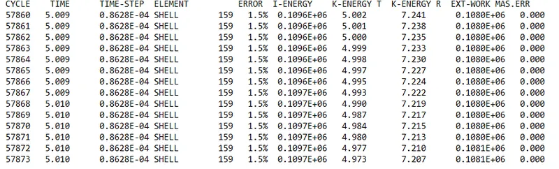
13. As the energy error is 1.5%, also the mass error is found out to be 0.000.

14.Click on The results to view them in animated format.

15.For the Graphical view use the Page window layout below the preferences option in Toolbar and split the screen according to the graph plots

16. Import T01 File from the Output file.

17. For Rigid wall, Forces choose Rigid walls > 1 punch> Total Resultant Force]

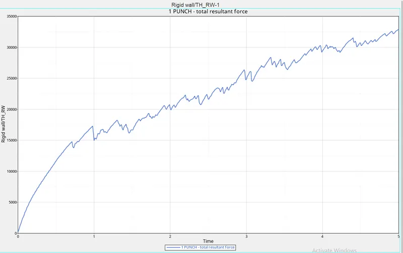
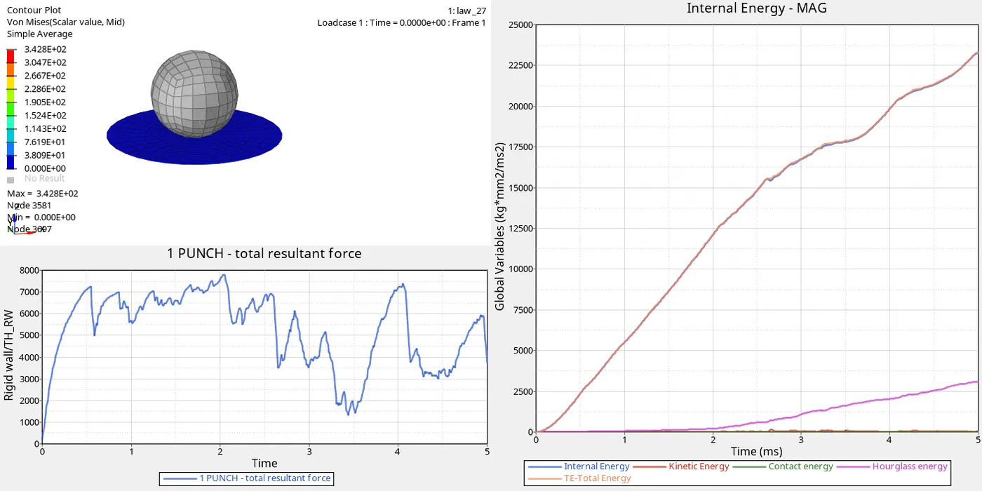
18. For the Energy graph choose the energies to be plotted, Global variables > Kinetic Energy, Internal energy, Contact energy, Hourglass energy, Total Energy > MAg, and choose to Apply.

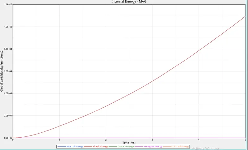
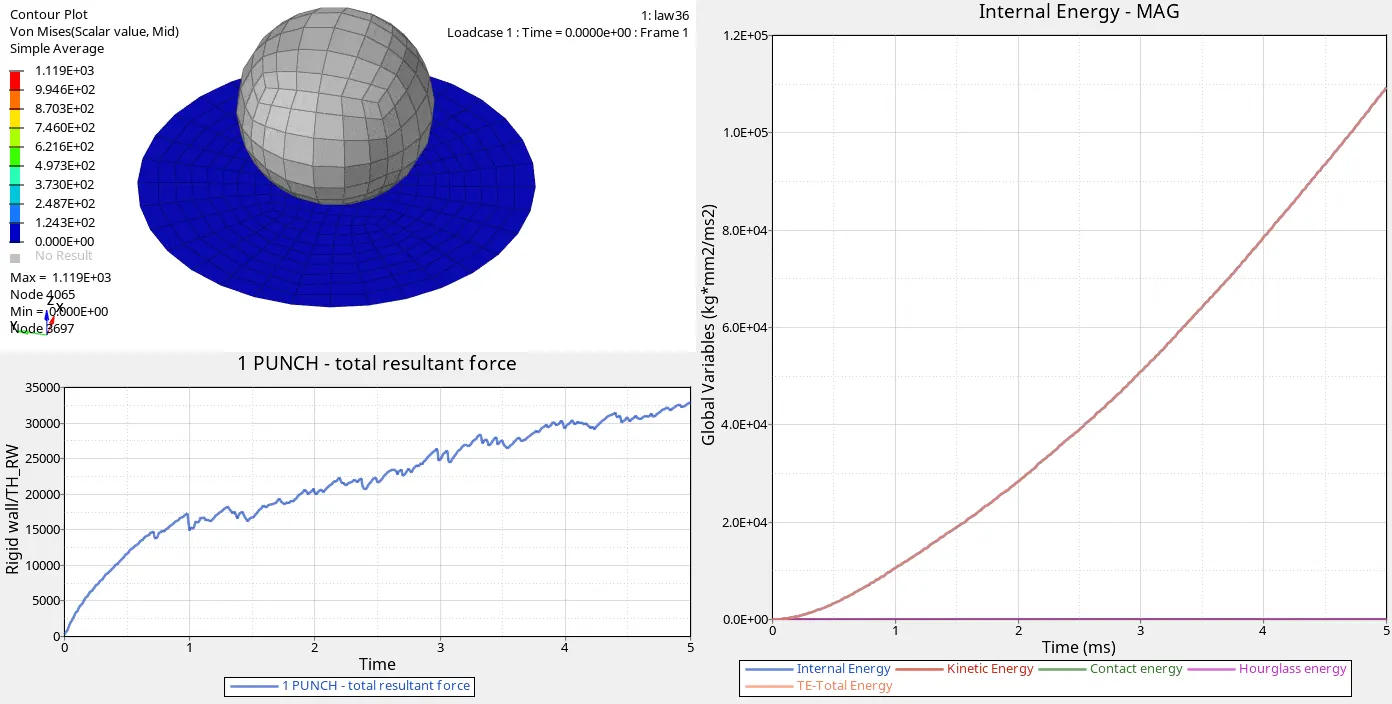
19.Case 2 & 7 Would represent the field scenario, in which case 2 with failure parameters such as IxFem, show realistic element split up. Law 36, which we give real stress-strain data to the solver to process, which can be closely related to field scenario too.

20. The Curve Obtained here is Bases on The real stress and strain data which can be directly Inputted to the solver.

Inference

• In this case, the Stress-Strain curve is defined from experimented values
• Law36 is applied; Elastic-Plastic - Tabulated
• Failure johnson card is defined
• The Elements are deleted during impact
• IxFem is 0 in this case so, failure criteria based on `epsilon` which is dependent on D1 D2 D3 values
• A higher curve leads to higher strain which is a faster failure.

RESULTS cONSIDERED:

CASE-1:

• Total no. of cycles=49380.
• Energy error=0.8%
• Mass error=0
• Simulation time (s)=56
• Material: Isotropic elastoplastic
• according to the given value of the youngs modulus as 710 GPA and sigma max as 425 no elements should be failed.
• because the failure rate is given as 15% element deletion occurs.

CASE-2:

• Total no. of cycles=49217
• Energy error=4.1
• Mass error=0
• Simu7lation time (s)=89s
• The same material was used only there is a change in the failure card.
• Isotropic elastoplastic with I_failsh=1, Dadv=1, IxFem=1.
• Comparing with the Previous case The element is getting cracked here and deletes after cracking.
• BY turning On IxFem=1, we can see the Crack propagation Clearly.

CASE-3:

• Total no. of cycles=49408
• Energy error=0.8
• Mass error=0
• Simulation time (s)=53s
• The failure card is deleted in this case.
• We can't control the rate of failure of the elements when It reaches Yield Point
• The element will Undergo Irregular element Deletion.

CASE-4:

• Total no. of cycles=49304
• Energy error=1.1%
• Mass error=0
• Simulation time (s)=54s
• In this case, we assigned Eps max=0, so the element will not fail until or Unless it crosses that value.
• Until or Unless specifying The EPS max value the Element Does not Fail
• So the Total energy Graph keeps Increasing.

CASE-5

• Total no. of cycles=47969
• Energy error=1.3%
• Mass error=0
• Simulation time (s)=52s
• In this case, Change The law as Elastic(Hookes's law), linear Deformation.
• As the Material behaves as elastic in Nature.
• The element doesn't undergo any crack or deletion.
• when the component crosses the Yield point the value obtained is known as the Garbage value.

CASE-6:

• Total no. of cycles=41113
• Energy error=-7.1%
• Mass error=0
• Simulation time (s)=44s
• In This case, the material law of the component has been Changed to Plast brittle (Law_27)
• The Brittle Material will undergo large stress and as soon as when it reaches the plastic Strain Region it Fails.
• It is a combination of Elastoplastic material.
• when it reaches the Yield point the elements will get collapsed and Deleted.

CASE-7:

• Total no. of cycles=57875
• Energy error=1.5%
• Mass error=0
• Simulation time (s)=62S
• In this case, assign law as 36 (Law_36 Plast tab)
• Here the element undergoes Lot of Strain
• The Eps values are defined by 3 cases
• the element starts failing in one case, element failing comes to end and gets deleted in another case.

CONCLUSION:

1. By the above Assignment I've gained knowledge About the Parameters To be considered while doing analysis.

2.Law 1 is used for elastic materials

3.law 36 and law 2 are mostly used in Industries.