Assignment 4
Objective:-
Compare 7 cases as discussed in last 3 slides, in a tabulated format on the basis of:
1. Total number of cycles, Energy error, mass error and simulation time.
2. Notice the animation of all 5 and describe the animations in brief on the
basis of whether the elements are being deleted or cracked.
3. Plot energies and notice any difference.
4. Based on all the results, which case would represent the on-field
scenario.
5. Prepare a ppt/docx and list down case by case result and your conclusion
as to why the failure happened.
Answers:-
1. Total number of cycles,Energy error, Mass error and simulation Time.
| Cases | File Name | Total number of cycles | Energy error(Min to Max %) | Mass Error | Simulation Time |
| 1 | Law2_Epsmax_failure | 49380 | -.6% to 1.3% | 0 | 91.36s |
| 2 | Law2_Epsmax_Crack | 49217 | -1.1% to 5.9% | 0 | 135.91s |
| 3 | Law2_Epsmax_nofail | 49408 | -.6% to 1.2% | 0 | 93.67s |
| 4 | Law2 | 49304 | -.6% to 1.2% | 0 | 95.54s |
| 5 | Law1 | 47969 | -.6% to 4% | 0 | 92.88s |
| 6 | Law36 | 49030 | -1.7% to .7% | 0 | 93.82s |
| 7 | Law27 | 49508 | -.6% to 1.1% | 0 | 94.11s |
2. Brief on the animations.
Case 1 :- Law2_Epsmax_failure
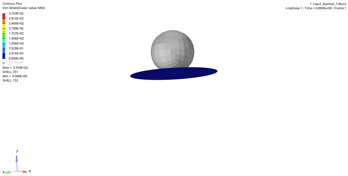 Side view
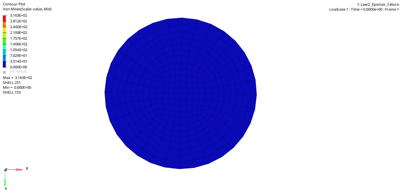 Bottom view
* This model is following Law2 failure (Johnson-cook failure model) . Failure of the element happens when one integration point reaches Eps_max . In this model we can see that the elements are getting deleted after the collision is taking place. Here we have zero as value for the Ixfem, this failure criteria will lead to element deletion instead of cracking. If we put contor in Von mises and none for averaging method the maximum stress is at 3.163E+02 and minimum is at 0. Here it takes about 5.0001ms to finish the run.
Case 2 :- Law2_Epsmax_Crack
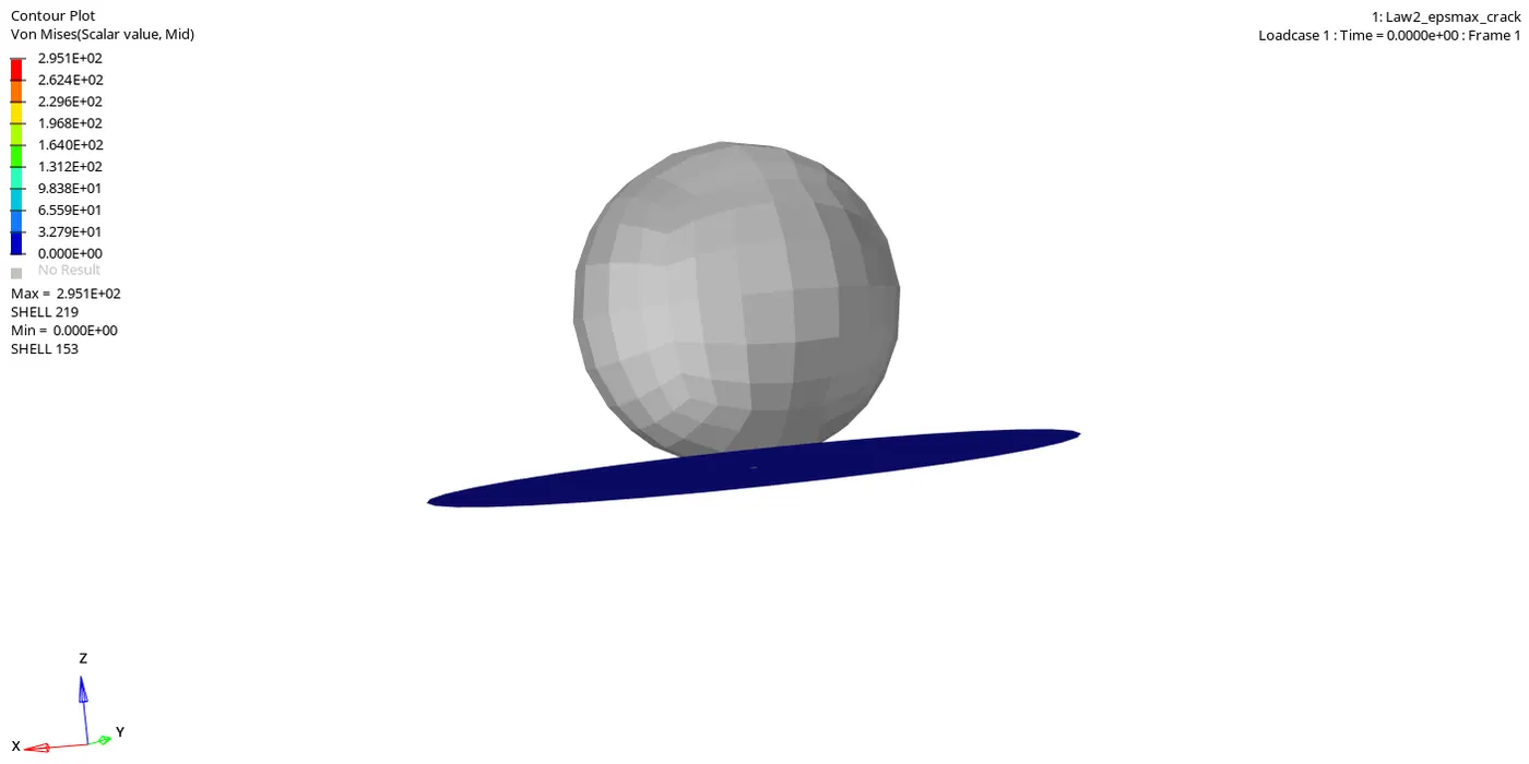
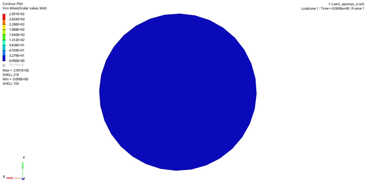
* In this model also we follow Law 2 but we have changed the value for Ifail_sh=1, Dadv=1 and Ixfem=1. We can see that the elements are getting cracked and then deleted in this model. The elements get deleted when the cracked element is again cracked. When we change the Ixfem=1, It will make the elements to crack instead of deletion. The Ifail_sh=1 tells when to fail, it will calculate the failing criteria on each integration point. Dadv=1 (It will be only active when Ixfem=1) This is the criteria for crack advancement, the propagation on the crack through out the model is found out by this. Here maximum stress is at 2.951E+02 and minimum is at 0. Here it takes about 5.0001ms to finish the run.
Case 3:- Law2_epsmax_nofail
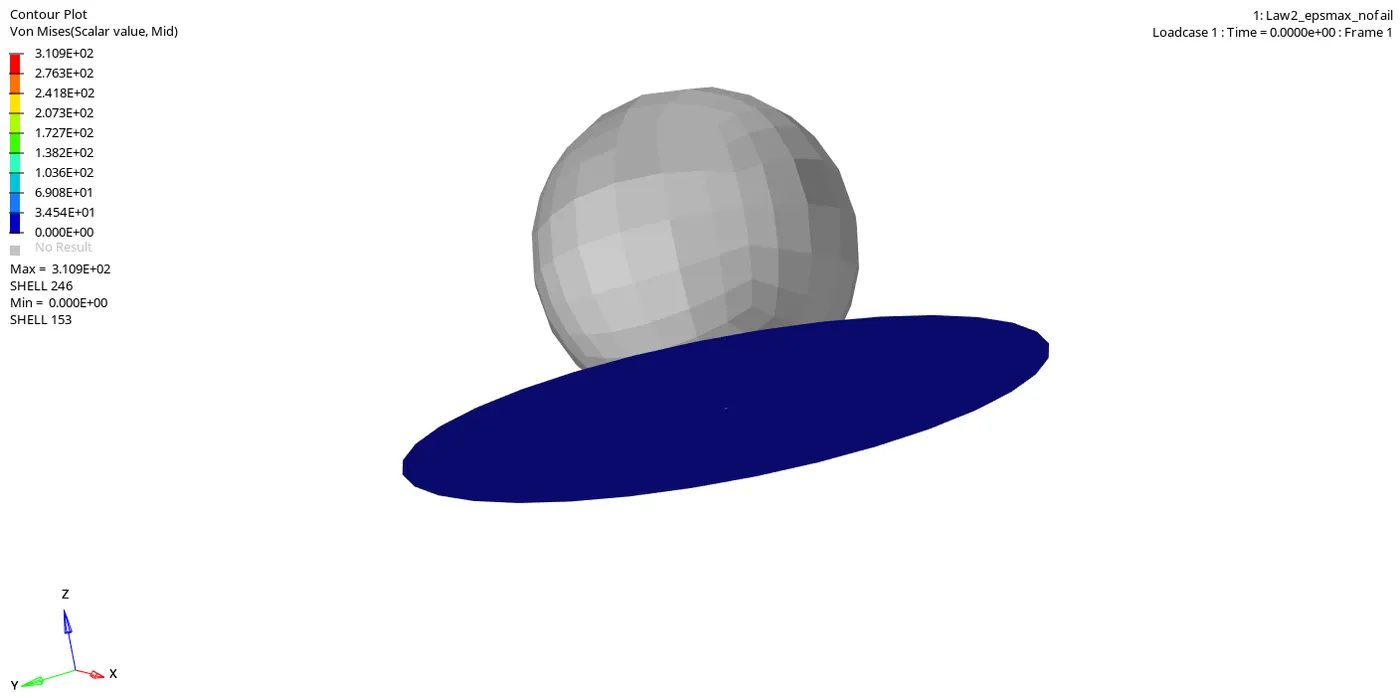
* In this model also we follow Law 2 but we have deleted the failure card. So the result of this simulation is almost same as the first case.The element wont crack they only get deleted as there is no failure card there will be no Ixfem value . But in everycase deleting the failure card wont give the same value for a case with the failure card. If there is no failure card the failing of an element is only based on Eps_max value and the result will not be based on realistic conditions.
Case 4:- Law2
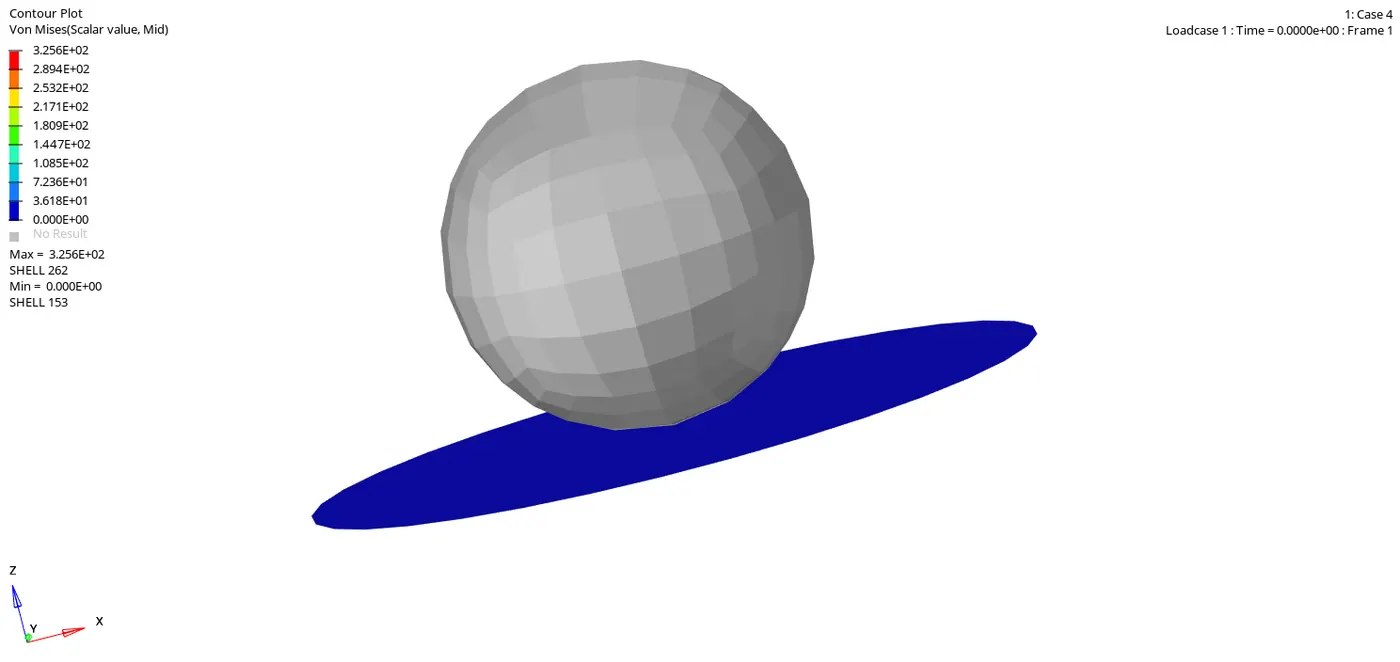
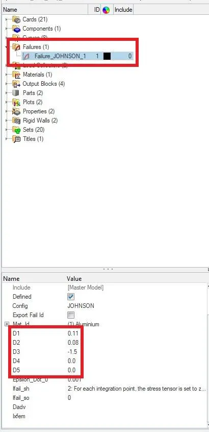
*In this case we can see that the Eps_max value is set to Zero. So the solver will use the default value, which ia about 10^30. this value is soo huge so that ith model will never fail. But still we can see that our model is failing and the elements are getting deleted. This is because even if we delete the Eps_max value there is failure card . In that D1,D2, D3 , D4, D5 values are inputed, with these parameters solver will solve the equation :-
 Thus find a condition to fail. Based on this the elements got deleted.
Case 5 :- Law1
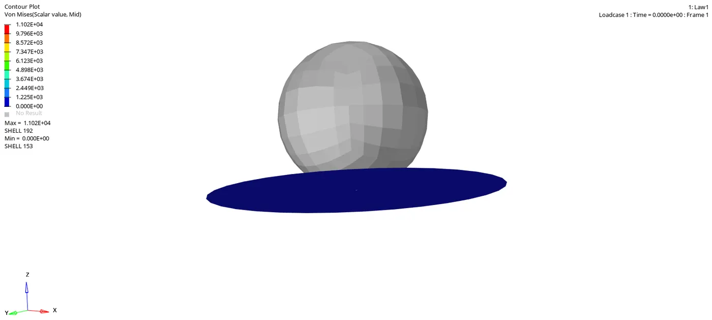
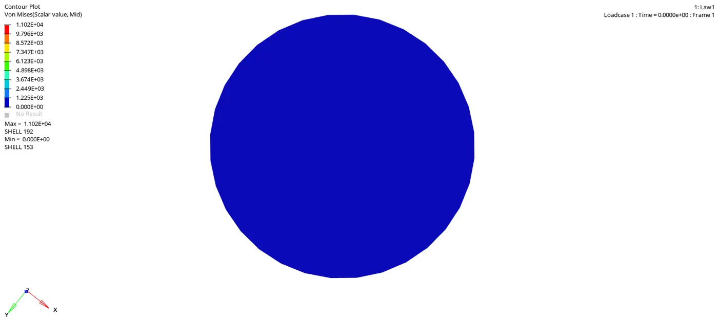
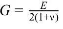
* Here in the material we have used Law 1, this law follows the Hooke's law of elasticity i.e a linear relationship between the stress and strain. The material stiffness is determined by Young's modules(E) and Poisson's ratio (n).
Here as the material follows hooke's law which in the elastic region no permanent deformation is occuring. The stress- strain curve follows a linear path. So no elements are failing,so no deletion of elements is present here.
Case 6:- Law36
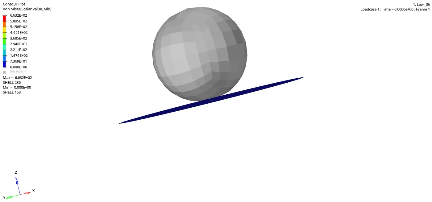
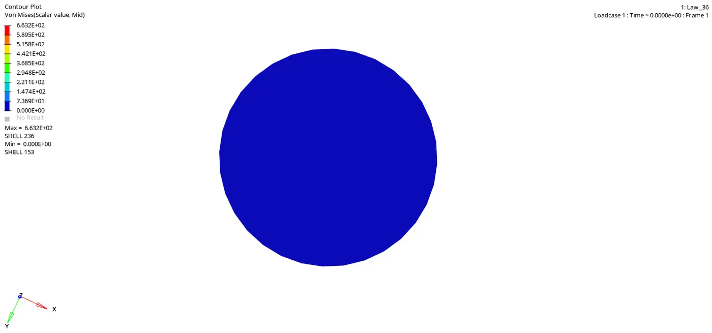
* Here Law 36 is used, This law helps in modeling isotropic elastro-plastic material using user defined funtions for the work hardening portion of the stress-strain curve for different strain rates. In this simulation we can see that the deletion of element from the centre is not starting like a square which is seen in other models. This is because this law will give use a more acurate result due to the input lab values.
Case 7:- Law 27
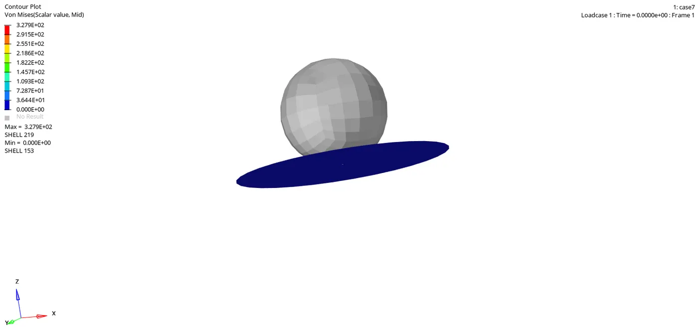
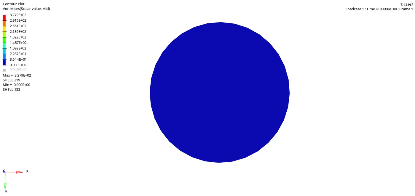
* In this simulation we have used Law 27, which is isotropic elasto-plastic material law with orthotropic brittle faliure model. So we can see in the simulation that after the ball is hitting the plate ,the plate is deformed and break like a brittle material. Here also element deletion take place.
3. Energy Graphs
Case 1 :- Law2_Epsmax_failure
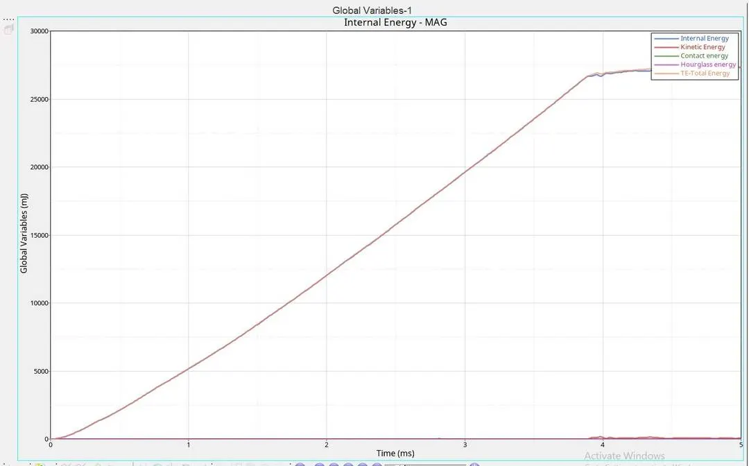
* The Hourglass energy is zero because we are using QEPH shell formation where the hourglass energy is reduced by perturbation method.
* The kinetic energy is zero at first because the plate is not moving at the beganing. After the ball is hitted and the material breaks then only the Kinetic energy comes in.
* The internal energy is zero at first after the collision some of the energy is absorbed by the plate and get deformed. This is why the internal energy is increaseing.
* The total energy is the sum of all energy that is why it growing with respect to time.
Case 2 :- Law2_Epsmax_Crack
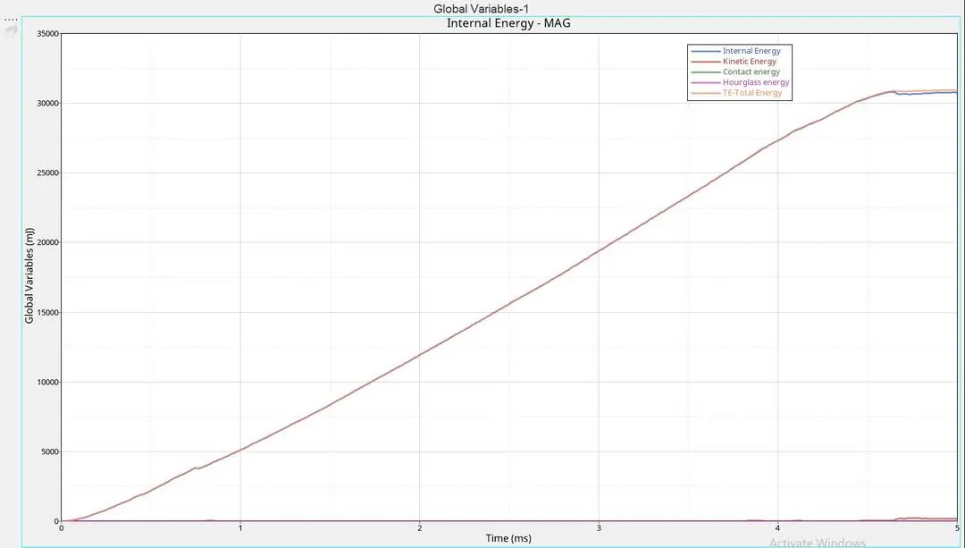
* Here also the contact energy and Hourglass energy is zero due to the usage of recommended shell properties
* The kinetic energy will increase from zero to a small value due to the collision and breaking of the plate.
* Internal energy is formed in due to the collision goes on increaseing.
* As kinetic and internal energy goes Total energy also increases.
Case 3:- Law2_epsmax_nofail
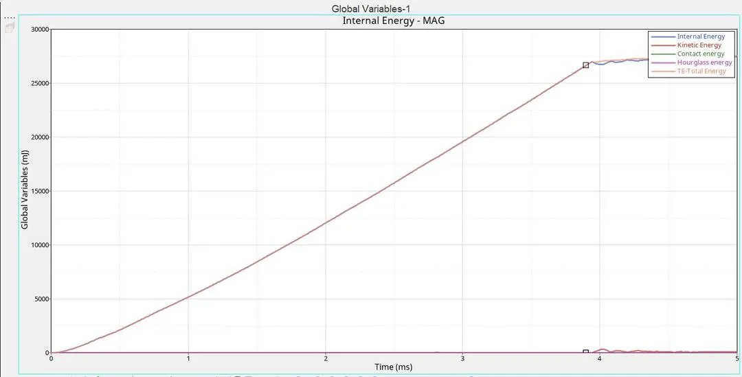
* The Failure card is deleted in this case, Based only on Eps_max the failing take place. So the values of the energy is having a change Compare to the graph in othe above case.
* The hourglass and contact energy is same as before.
* The collision is giving kinetic and internal energy. Results in the increase of total energy.
Case 4:- Law2
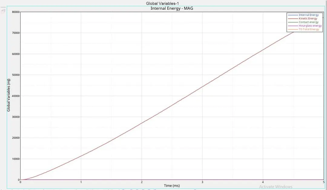
* Here the Eps_max value is deleted. so the solver takes a higher value . So the material will only fail at a higher range of energy.
* The propagation of enegries are same as the other with respect to time.
Case 5 :- Law1
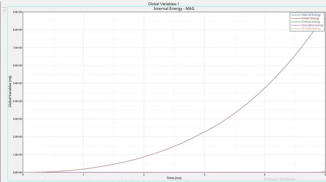
* We use Elastic law in this. So from the graph we can see that the material is not gonna fail.
*As the recomended shell properties are used there is no hourglass effect.
* Kinetic energy and internal energy is increaseing. Thus total energy also increases.
case 6:- Law36
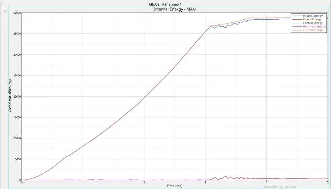
* Here we can see that when the collision happens the hikes and dips in curve are more compare to other graphs this is because the values given to the solver is the values that we get from the lab.
* This curve will be more Accurate than the other ones.
Case 7:- Law27
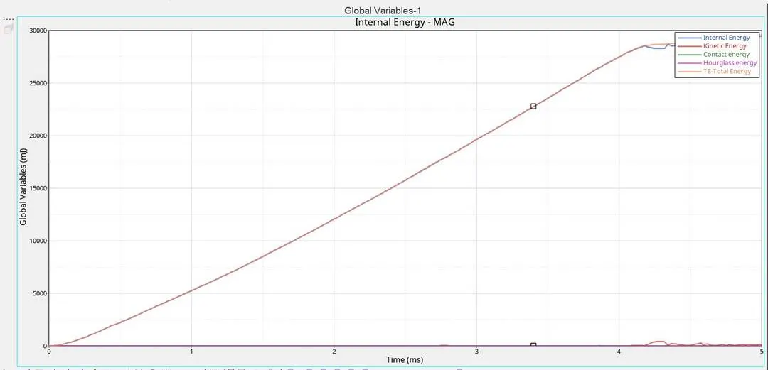
*The Law 27 is based on brittle faliure property.
*Here Also Hourglass is not present due to the QEPH Formulation.
*Kinetic energy and internal is increaseing with respect to time. Thus the total energy is also increaseing with them.
4. which case would represent the on-field scenario ?
Law 36 :-
* In Law 36 we are getting a energy error of about -1.7% to .7%, Which is acceptable as both are nearer to zero.
* Also in this law the values that we are inputing is the values we get from the lab. which is based on real experiments.
* The work hardening portion which is the plastic region is created from the lab values and the elastic region can be made by giving the young's modulus and poisson's ratio.
* Thus due to these reasons the Law 36 is more similar to real life compare to others.
5. Conclusion
Case 1 :- Law2_Epsmax_failure
* In this we are runing the file as same as it is given
* Law 2 (Johnson-cook material) is used.
* This law represents an isotropic elasto-plastic material using the johnson-cook material model.
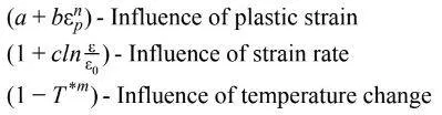
* Model expresses material stress as a function of strain, strain rate and temperature.

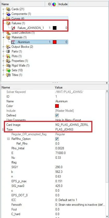
* Based on the Faliure card and Eps_max values the model will fail here.
Case 2 :- Law2_Epsmax_Crack
* Here for the same file above with law 2 is used again
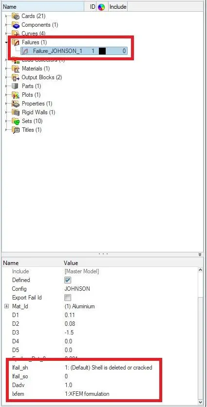
* In this we have changed the value for Ifail_sh=1, Dadv=1 and Ixfem=1.
* This will only affect the Visualisation of the simulation.
* These values will show the simulation more correctly by showing the crack and crack propagation.
Case 3:- Law2_epsmax_nofail
* Here the file is run after deleteing the Johnson cook failure card.
* As the failure card is not present the failing of the elements is fully based on Eps_max value.
Case 4:- Law2
* Here the Eps_max value is deleted
* The default Eps_max value will also give improper result.
* But the presence of Failure card will help us to get a better result in this case as the D1, D2, D3, D4 and D5 values are inputed.
Case 5 :- Law1
* The Law 1 is applied to the material card here.
* This law is about Linear elastic material, elasticity law follows the hooke's law of elasticity i.e a linear relationship between the stress and strain.
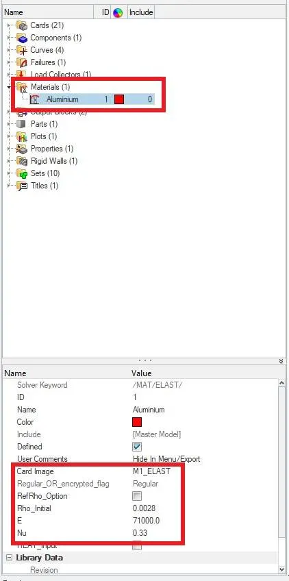
* The material stiffness is determined by young's modulus of elasticity (E) and Poisson's ratio(n).
* In this case the Young's modulus, density and poission's ratio is inputed to the solver here.
* This model's and elements wont fail as it is following elastic law.
case 6:- Law36
* The Law 36 Material law helps in modeling isotropic elasto-plastic material using the user defined funtions for the work hardening portion of the stress-strain curve for different strain rates.
* The curve defined is nothing but the stress-strain curve after the yield point. the yield point is set to '0'
* In case 6 we need to change the Law to 36.
* Also input the values as given below.
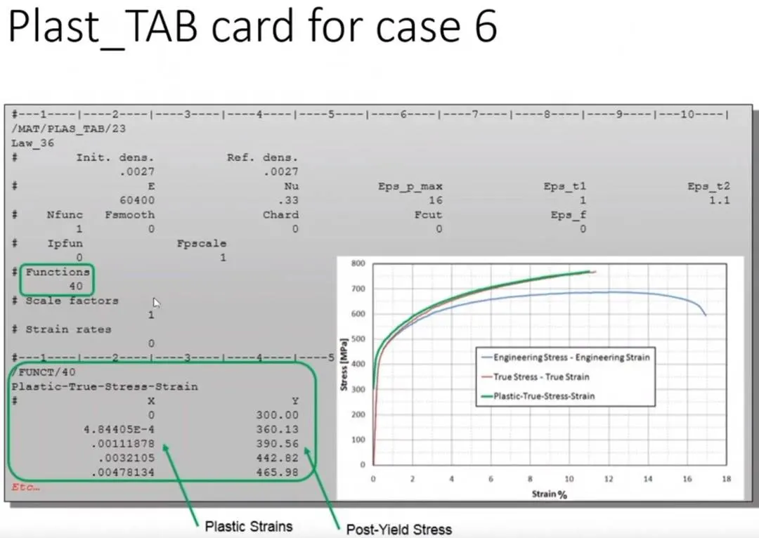
* Also plot the curve graph with the values in the above slide.
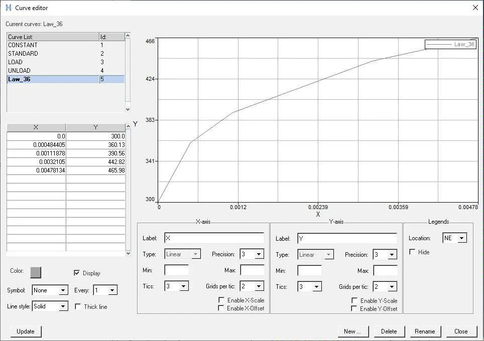
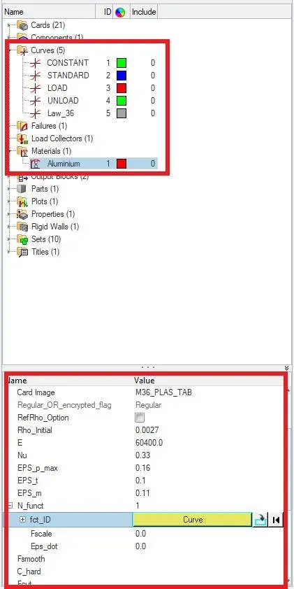
* Here we get the result based on the values that we input on the curve.
Case 7:- Law27
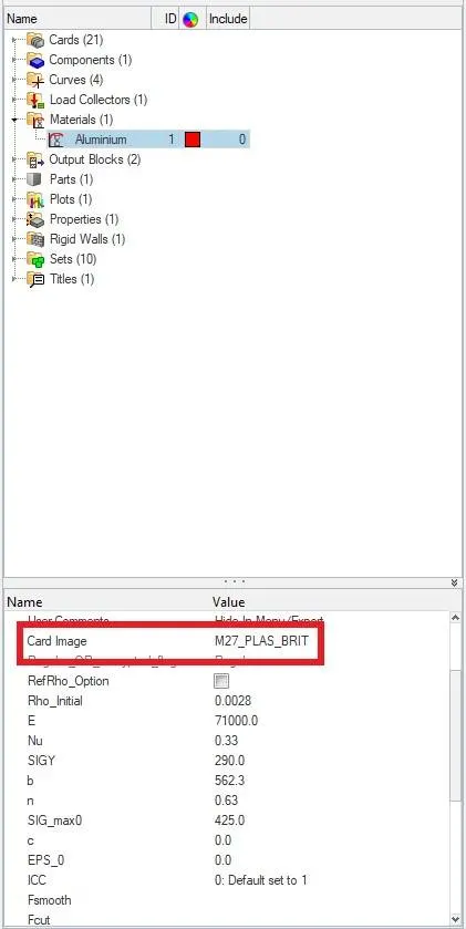
* This law 27 has isotropic elasto-plastic material law with orthotropic brittle failure model.
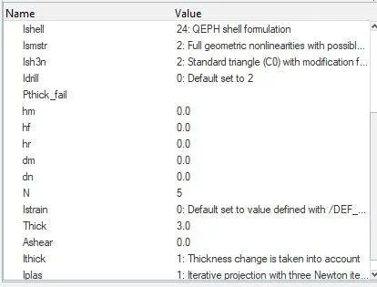
* In this case we need to open the LAW27_000.rad file and change the shell properties to recommended shell properties
* Here the plate will be having more brittle nature.
Result:-
All 7 cases have been run on the solver as per the given conditions and the observations & conclusions are recorded.