Assignment 3

Skill lync assignment 3

Objective: The objective of this assignment is to run a simulation for the given starter and engine files after editing the engine file. The simulation is then to be checked for hourglass energy error and other such errors, and then re-run after modifying the element properties.

Theory: Hourglass is an apparent phenomenon of component distortion with zero strain energy, .i.e. no strain or stress generated. The hourglass energy associated with this phenomenon arises purely from the inaccuracies of the FEA process, particularly from the under-integration over the FE elements due to inadequate number of integration points. In order to properly run a simulation with acceptable accuracy, hourglass energy has to be minimized as much as possible.

There are a variety of ways to minimize such an error, as are discussed below.

• The most obvious solution is to reduce the element size, i.e. make the FE mesh finer. This reduces the error per element. However, this is not viable in the case of crash analysis, since reducing the element size also reduces the time step required for modelling the crash.
• In case of simulations with relatively high linear velocities of elements, viscous damping can be used. Here, an artificial force is applied to element nodes to counter the hourglass energy caused by the element velocity. In this method, the hourglass needs to be detected before the method is used. Viscous damping is only recommended when expected hourglass energy is very large in magnitude.
• Another method is artificial material stiffening that absorbs the hourglass energy. This method deals with hourglass energy before it arises. However when this method is used, there is a possibility that computed values of strain may be inaccurate due to the modified material properties.
• Under-integration in an element happens due to a reduced number of Gaussian integration points over each element. Such elements are usually chosen to save on computing cost and thus reduce computational time. Therefore, the surefire way of eliminating hourglass energy is to incorporate full integration by means of elements with all the necessary number of integration points.

Case setup 1: The files provided are a pair of .rad files, one being a starter file and an engine file for a rail component. The engine file is edited so that simulation run time is 55 ms. The number of animation steps are adjusted to 25.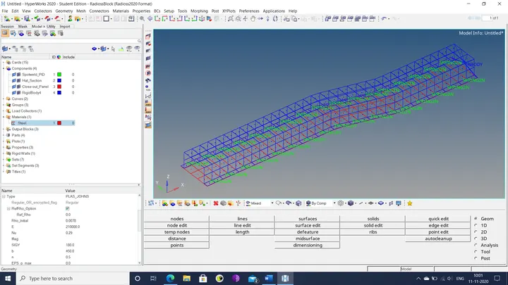

Figure 1: Imported starter file

Case setup 2: The files have two more copies made with the same simulation run time and animation steps. The difference in these files are that elemental settings are changed to the following, so that hourglass energy and other such errors are changed. Number of animation steps is also increased to 60.

Parameters		Comment
Ishell =24		QEPH 4 nodes shells are best combination of cost and accuracy.
Ismstr=2		Full geometric nonlinearities (default)with possible small strain formulation activation in RADIOSS Engine.
Ish3n=2		Standard 3 noded shell (C0)with modification for large rotation(default)
N=5		Number of integration points set to 5 for accuracy bending.
Ithick=1		Thickness change is taken into account for accuracy.
Iplas=1		Iterative plasticity for good accuracy.

Procedure: The simulation is setup via the following sequence of steps.

1. A copy of the engine file is edited so that total runtime (listed under the /RUN section) is 55 ms.
2. Under the /ANIM/DT section, the number of animation steps are set to 25 by setting the time step that is run time divided by number of animation steps (55/25), i.e. 2.2 ms.
3. The starter file is imported into the hyper-works workspace by the import>solver deck option.
4. The simulation is run by the analysis>RADIOSS option.
5. The resultant output files are exported to a separate file.
6. The hourglass energy error and mass error are listed in the .out version of the engine file, as shown below.

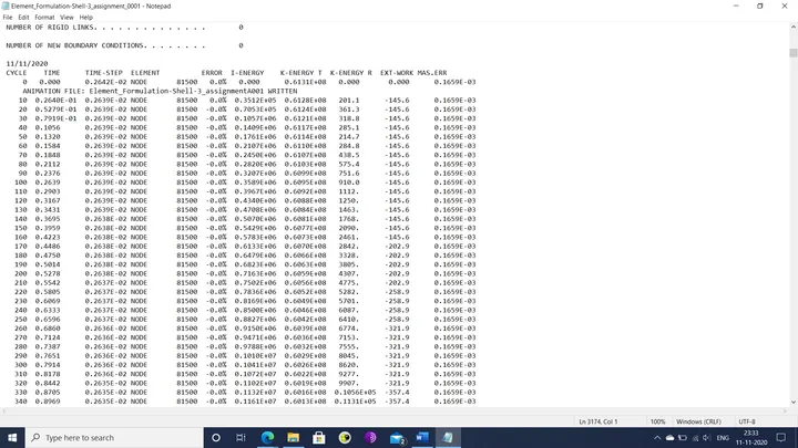
Figure 2: Case 1 output file

Here, the hourglass energy error reaches a mimimum value of -10.3% and the mass error remains constant at 0.166%.

7. The hyper-view workspace is then opened and then the .h3d file generated by the RADIOSS simulation is imported here.
8. The 1 dimensional elements, i.e. spot welds are represented as dots via the preferences>options>visualization menu, as shown below.

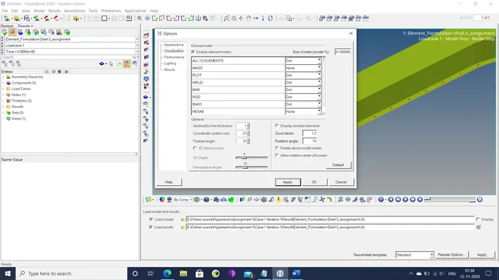
Figure 3: Spot weld visualization

9. The contour button is used to show the hourglass energy contour on the component animation, as shown below.

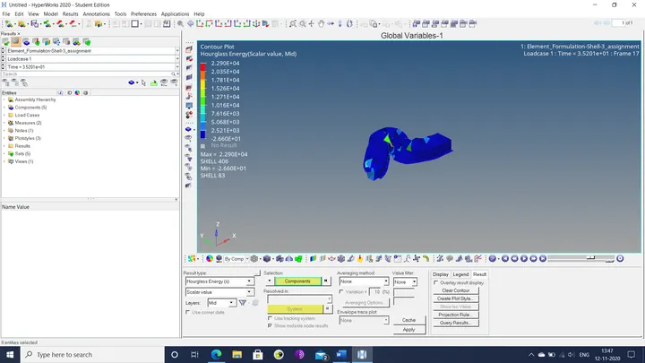
Figure 4: Hourglass energy animation

10. A parallel window is opened, where the hyper-graph 2D workspace is loaded, as shown below.

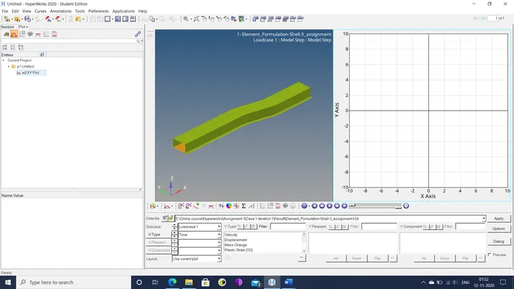
Figure 5: Split window display

11. The file Element_Formulation-Shell-3_assignmentT01 file is imported into the hyper-graph 2D environment and the contact energy is plotted, which is shown below.

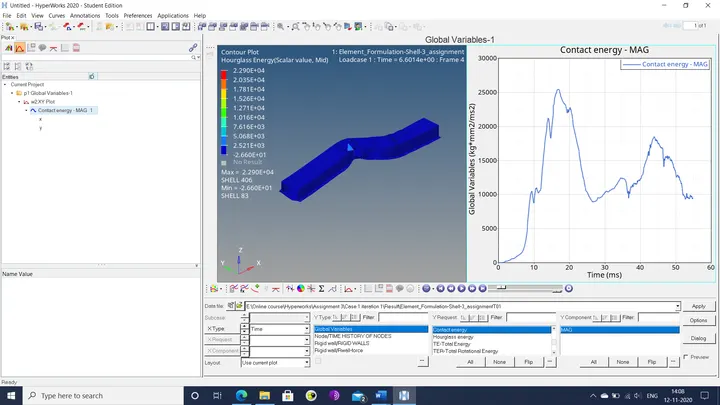
Figure 6: Contact energy graph

12. In a similar manner, the hourglass energy, internal energy and total energy are plotted in the same window, as shown below.

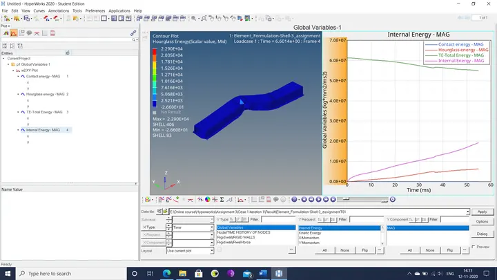
Figure 7: Multiple energy graphs

13. A new plot is opened where the wall forces are plotted, as shown below.

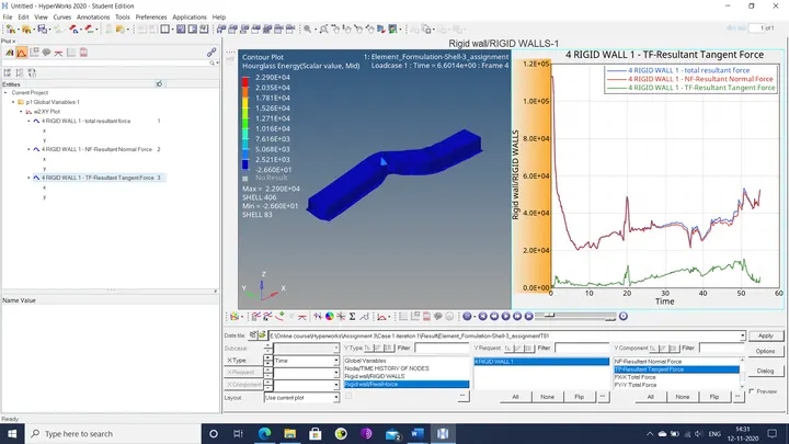
Figure 8: Rigid wall forces

14. The second copy of the starter file is imported into the hyper works workspace.
15. Here, the necessary properties to be modified as mentioned in the case setup are identified in the property card and changed accordingly.

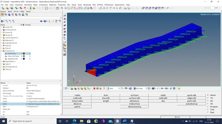
Figure 9: Imported file with modified element settings

16. The simulation is then run by the analysis>RADIOSS option with files being exported to a separate file.

17. In this case, the mass error is same as the first case, but the hourglass energy error does not drop below 0.1%.

18. Steps 6 to 12 are repeated for the second case. The resultant graphs are shown below.

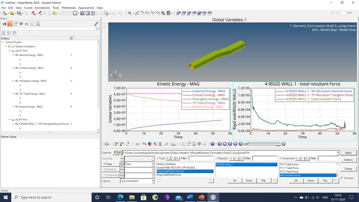
Figure 10: Case 2 graphs

Result: The two versions of the starter files have been used in 2 separate simulations to show the difference made by proper element settings.

• In case 1, the amount of hourglass energy was significant enough to be absorbed from the total energy.
• In case 2, the hourglass energy was almost completely eliminated. As a result, the drop in kinetic energy can be corelated to the rise in internal energy. The total energy is almost completely conserved within the system.
• Wall forces are reversed towards the end of the simulation in case 2.

Conclusion: The given starter and engine files are used suitably in simulation and the difference caused by the change in element properties are reflected adequately in the resultant graphs.