The effect of various shell element properties in Radioss on the simulation results of the crash scenario of rail against the rigid wall:

Comparing the simulation results of various shell element properties in Radioss for the crash scenario of rail against the rigid wall:

Objective:

The objective of this project is to simulate the crash scenario of the rail against the rigid wall using various shell element properties in radios. The effects of various shell element properties are studied and the best combination of shell element properties will be determined based on the simulation results.

Procedures:

Case 1 – Simulation with the given shell element properties:

• Import the given starter input deck file of the Radioss. The file can be imported using the “Import Solver Deck” from the “File” menu or using the shortcut icon in the toolbar.

  

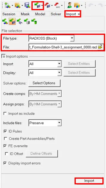
  Fig 1.1: Import solver deck

  Choose the file type as Radioss and select the required file name.

  

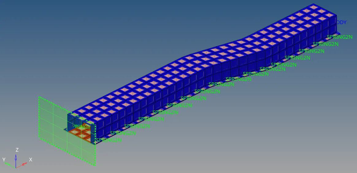
  Fig 1.2: Model of Original_Shell_Element_Formulation_0000.rad

• The starter input has all the model information including the shell element property.

  

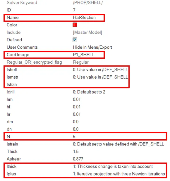
  Fig 1.3: Shell element property of hat section

  

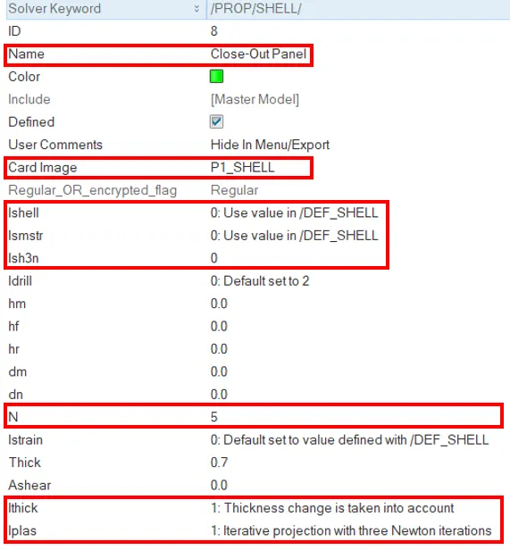
  Fig 1.4: Shell element property of close-out panel

  The important properties of the shell elements are as follows:

  Ishell: This parameter is used to select the element formulation for the 4-noded shell element i.e. quad element. Ishell can be 1, 2, 3, 4, 12, or 24. Ishell of 1, 2, 3, or 4 represents the Q4 element, which is an under-integrated Betytschko & Tsay formulation with options on hourglass treatment. Ishell of 12 represents the QBAT, which is a fully integrated element. Ishell of 24 represents the QEPH, which is an improved under-integrated element with physical hourglass stabilization. The default is Q4 element. It is an under-integrated element, it has only one integration point in the middle, and therefore there will be a high probability of hourglass effect. The element of QABT is a fully integrated element. Even though it won’t have hourglass effect the simulation time is high. The element of QEPH is a best compromise between the cost and the quality.

  Ish3n: This parameter is used to select the element formulation for the 3-noded shell element i.e. tria element. Ish3n is 2, which is a standard triangle (C0) with modifications for large rotation.

  Ismstr: Strain formulation of the element. The strain formulation can be 1 (small) or 2 (large) strain formulation. The default is large strain formulation.

  N: This parameter represents the number of integration points through the thickness. Default value is 0 and the N can be in the range of 1 to 10.

  Iplas: This parameter choses the calculation method in the plastic region. This parameter can be 1 (iterative projection with three newton iterations) or 2 (radial return). The default is radial return method. The suggested method for calculation is iterative projection with three newton iterations, as it gives more accurate result.

  Ithick: This parameter choses whether the thickness change has to be considered or not. The value of the parameter can be 1 (thickness change is taken into account) and the default value of 2 (thickness is constant). The recommended value is 1.

  For this simulation, the parameters from the starter input deck is used without making any changes. When the values are specified as 0, the values from the /DEF SHELL card is used.

• Change the run time to 55 ms in the engine input file. The run time in engine file can be edited directly or in the “Solver browser” of the Radioss.

  From the “View” menu activate the “Solver” deck from the “HyperMesh Browser”.

  

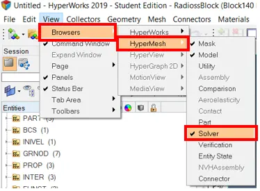
  Fig 1.5: Solver deck

  In the solver there is a separate drop down menu for the “Engine_Keywords”.

  

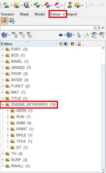
  Fig 1.6: Solver deck

  For editing /RUN card, go to /RUN drop-down menu and insert the new termination time in the editor.

  

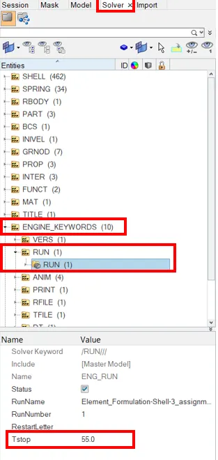
  Fig 1.7: Edited run time

  Thus by changing the run time, the simulation will terminate at 55 ms.

• Then the number of animation steps is changed to the minimum of 25 and maximum of 60. This can be changed at the /ANIM/DT card of the engine input file.

  /ANIM/DT card is edited at the /ANIM drop-down menu

  

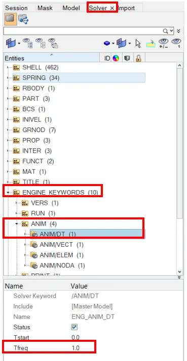
  Fig 1.8: ANIM/DT Edited

  Since the maximum number of animation is 60 and the termination time is 55 ms, the t_freq = 1 ms is used to get totally 55 animation step.

• The required results has to be selected in the solver browser, so that it has to be included in the engine input file. The required results can be selected either in the vector category or the element category. The results can be selected /ANIM/VECT and /ANIM/ELEM cards of the engine input file.

  /ANIM/VECT and /ANIM/ELEM cards are edited at the /ANIM drop-down menu

  

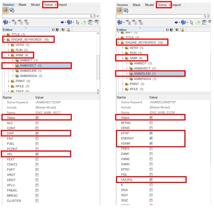
  Fig 1.9: Results included in the engine input file

  In the vector category, velocity and the displacement vectors are selected and in the element category the animations of the plastic strain, energy, von mises stress and the hourglass energy are selected for viewing.

• The starter input deck is then exported along with the engine file. This file is required for the simulation. Therefore, these files are exported first. Select the required folder on which these files has to be saved and give the required file name as the format of “FILE_NAME_0000.rad”. Select the “Auto export the engine file” option, therefore the engine input file will be automatically exported as a separate file.

  

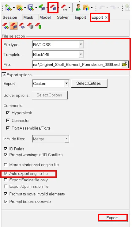
  Fig 1.10: Export the starter input deck and the engine input file

• After exporting the file, the file is run in the Radioss. The simulation is run using Analysis → Radioss option.

  

  Fig 1.11: Run the analysis in Radioss

  

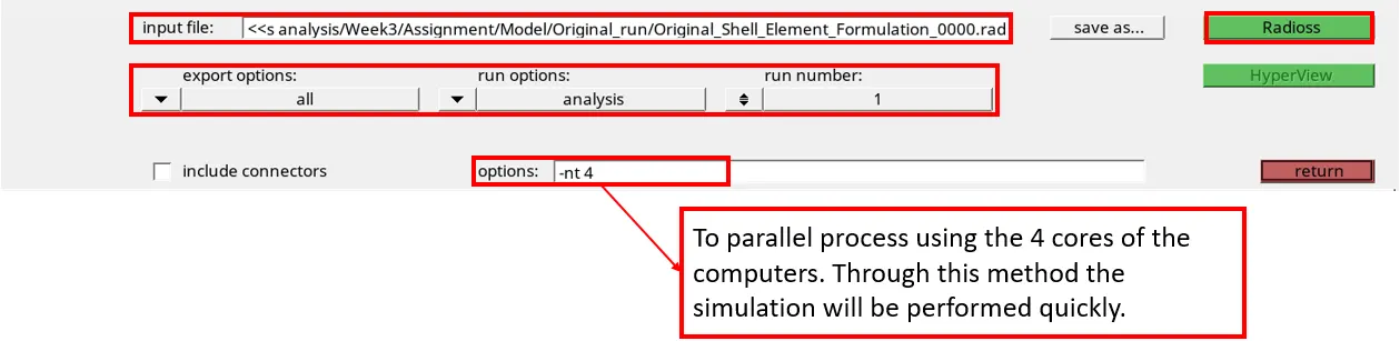
  Fig 1.12: Run the analysis in Radioss

• The progress of the simulation can be viewed in the displayed “HyperWorks Solver View”. This window shows the current time step, total time of the simulation if completed, memory consumed etc. and from through this the result files can be viewed.

  

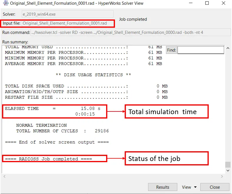
  Fig 1.13: HyperWorks Solver View

• The output file is checked for the accuracy of the result by checking the energy and the mass error during the simulation for each time step and the error at the end of the simulation.

  

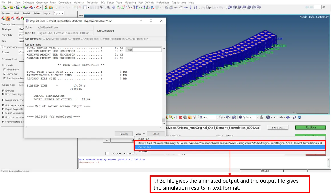
  Fig 1.14: HyperWorks Solver View – Output files

Output Description:

The energy error and the mass error due to the addition of the mass is checked in the output file “Element_Formulation-Shell-3_assignment_0001.out”.

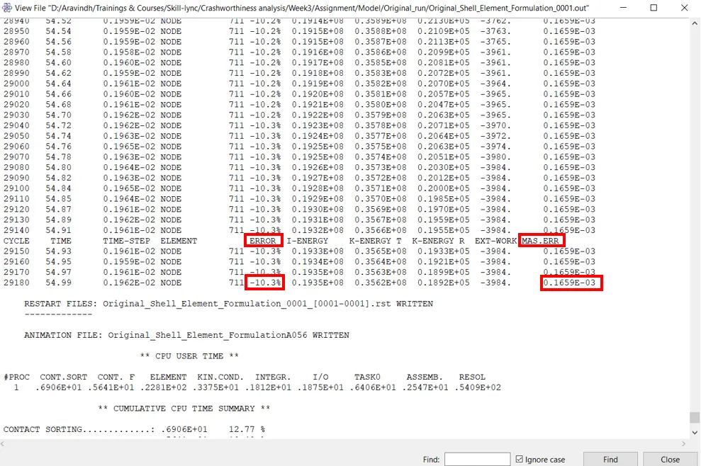
Fig 1.15: HyperWorks Solver View – Output files

The energy error is calculated in percentage using the formula:

`% Err = 100(frac{E_k + E_i + E^r_k}{E_(k,1) + E_(i,1) + E^r_(k,1) + E_(wk) - E_(wk,1)} - 1)` (Altair Engineering, Inc., 2019)

Where, E_k – Translational kinetic energy at current time

E^r_k – Rotational kinetic energy at current time

E_i – Internal energy

E_wk – Work of external forces (energy brought to the system)

E_,1 – Initial energy (at t = 0)

The hourglass energy is not considered for the energy balance (Altair Engineering, Inc., 2019).

The energy error must be in the range of -15% to +5%. Negative error means, the energy is dissipated from the system. Negative error means, the energy is created in the system. Positive error within 5% is acceptable. More than that there is some problem with the system. Numerical energy creation (not present in the physical sense) will lead to the wrong simulation result. There are many reason for the numerical creation of the energy in the system. One of the reason is the initial penetration during the contact interface definition. The positive energy error must be rectified immediately.

The energy error from the result of the end of the simulation is -10.3%. It is within the acceptable range. The reason for the energy error is due to usage of the Betytschko & Tsay under-integrated shell element for the simulation. Since, this is the under-integrated element, which has only one gauss quadrature point, there is an hourglass associated with the simulation. Since this hourglass is not considered for the energy balance, it adds to the energy error.

The mass is added due to the Interface TYPE2, Spot_flag = 1. This mass is added initially at t = 0 (Altair Engineering, Inc., 2019).

The mass added should be large and it should be large locally, since it will lead to the false simulation result. The mass error from the simulation is 0.1693E-03%. Therefore the mass error is also small, indicating that the added mass is not very large.

Since the energy and the mass errors are within the acceptable range, the other results are checked.

The results such as animation and the time-history plot can be viewed by accessing the .h3d file directly through the HyperWorks Solver View, by selecting the “Results” option. This option will open the HyperView window directly where the simulation results can be post-processed.

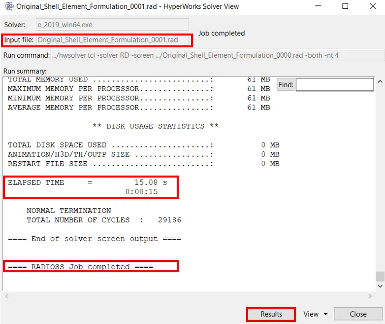
Fig 1.16: HyperWorks Solver View – viewing result in HyperView

In the HyperView window, load the model and the result file (.h3d file) and play the animation at the required view.

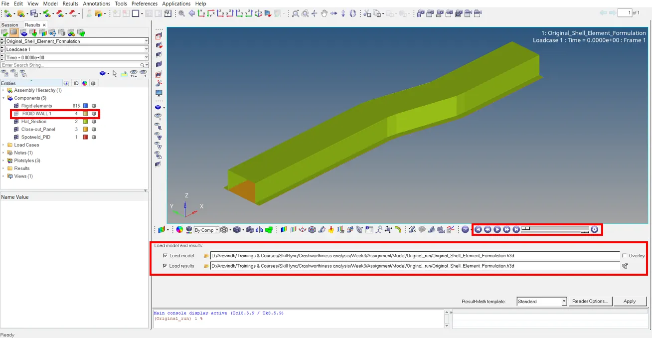
Fig 1.17: HyperView – post-processing the simulation results

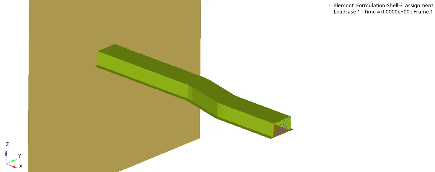
Fig 1.18: Result along with the rigid wall

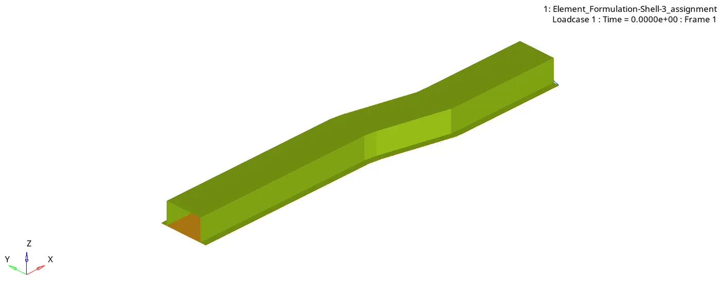
Fig 1.19: Result without the rigid wall

The rail is completely destroyed and there are many elements with hourglass deformation. The contours of the Von-Mises and plastic strain tensors are viewed to get more understanding of the behavior.

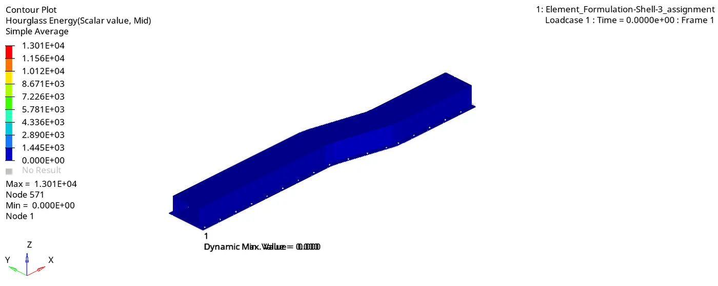
Fig 1.20: Animation of Hourglass energy

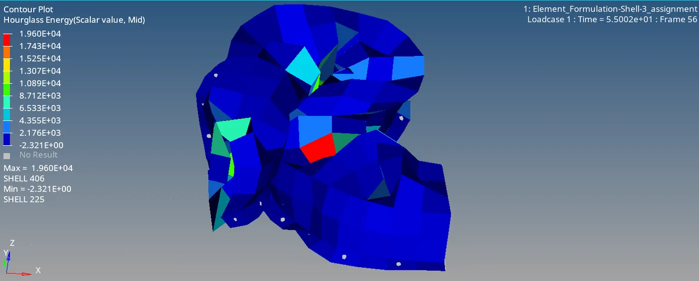
Fig 1.21: Hourglass energy at t = 55ms

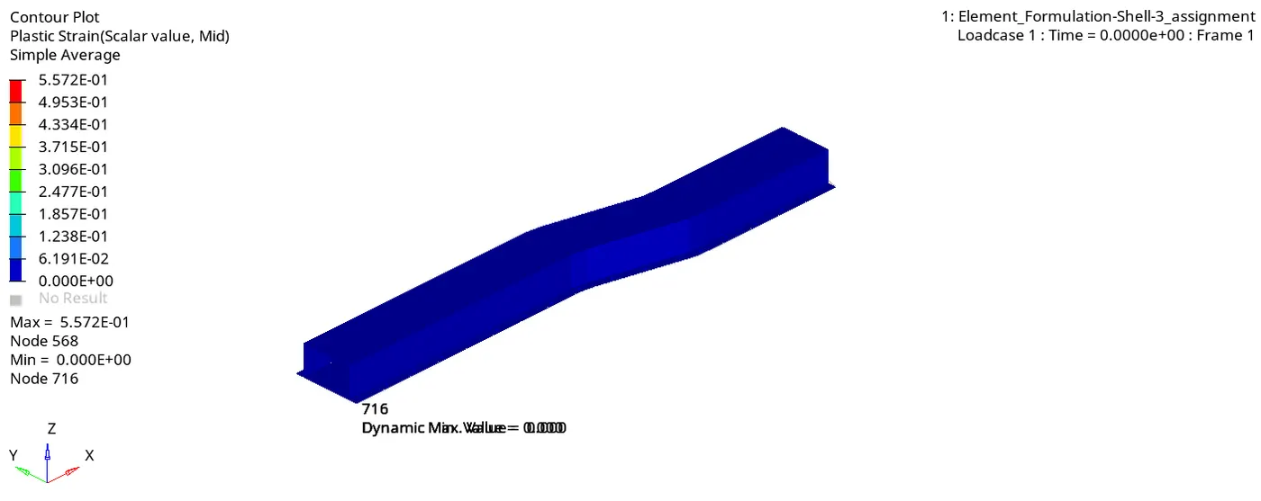
Fig 1.22: Animation of plastic strain

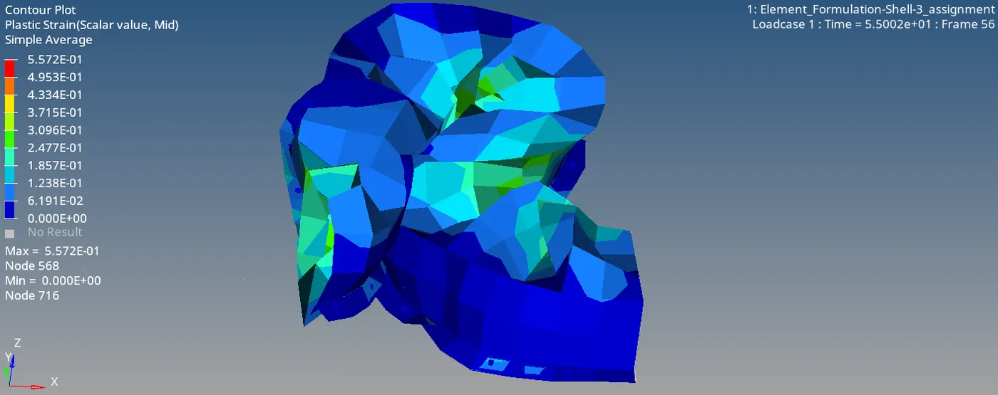
Fig 1.23: Plastic strain at t = 55ms

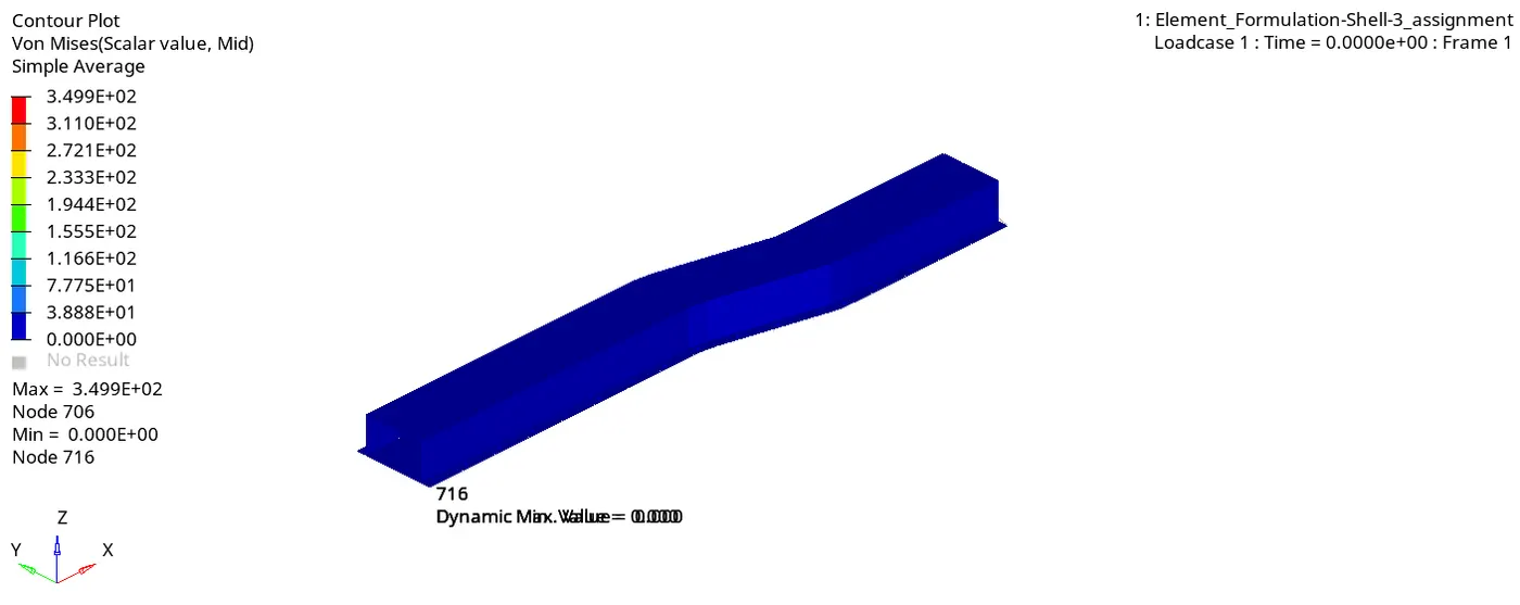
Fig 1.24: Animation of Von-Mises stress

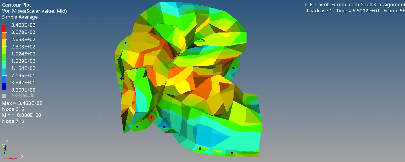
Fig 1.25: Von-Mises stress at t = 55ms

The time-history plot results of the simulation are viewed to know the graphical results of energies, forces etc. through the various time steps of the simulations. This graphical representation shows clearly any deviation from the expected or experimental results.

For viewing the graphical results, HyperGraph has to be used. Divide the current HyperView window into two and open the HyperGraph in the new window.

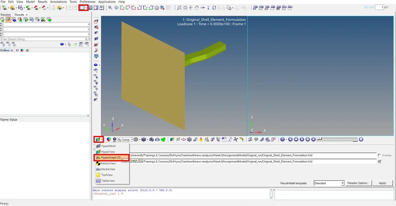
Fig 1.26: Dividing the window and opening HyperGraph

The .T01 file (time-history result file) of the simulation is opened.

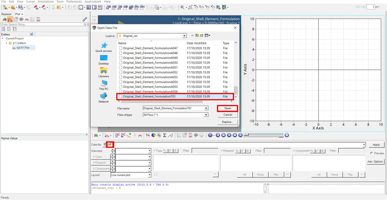
Fig 1.27: Opening .T01 file in HyperGraph

Then the required graph type, graph variables are selected. The HyperView asks for the required unit system in which the results has to be viewed. The same unit system in starter input deck with millimeter for length, millisecond for time and gram for mass is selected. The HyperGraph will show the time-history plot in that unit system.

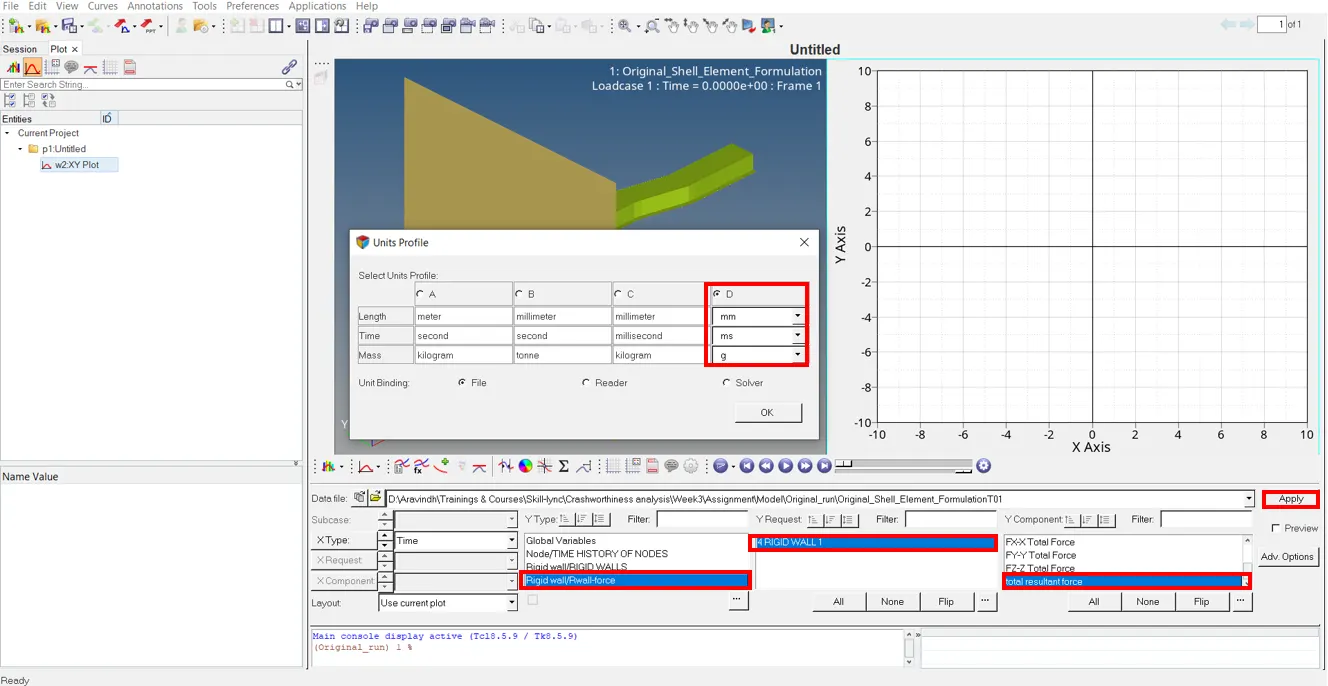
Fig 1.28: Loading the required graph in the required unit system

The time-history plot of rigid wall forces such as total resultant force, tangential and normal resultant forces and the energies such as internal, kinetic, contact and the hourglass energy are plotted.

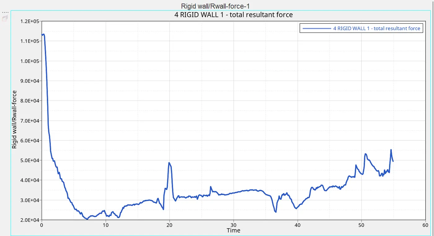
Fig 1.29: Rigid wall force – total resultant force

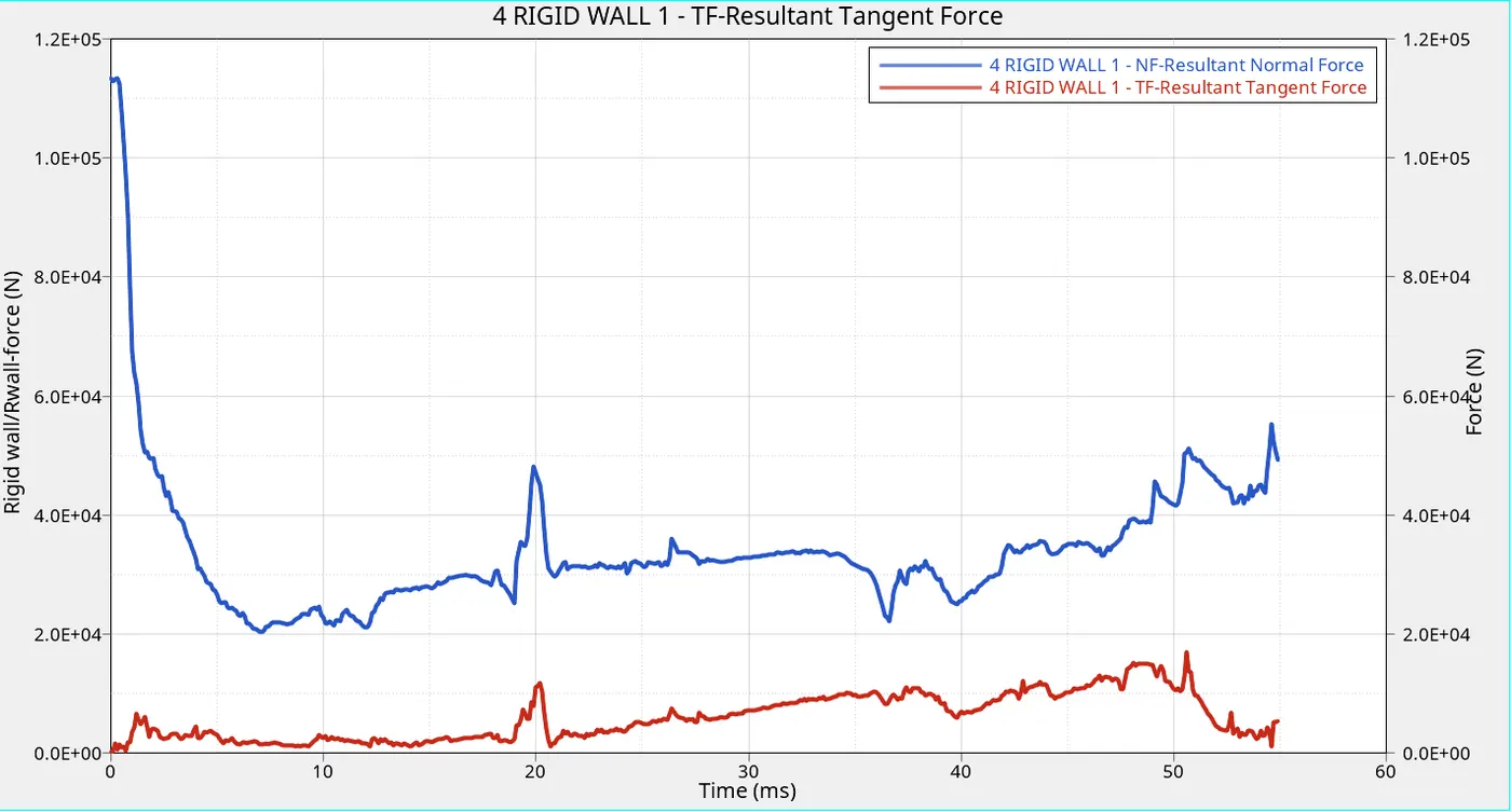
Fig 1.30: Rigid wall force – normal and tangential resultant force

From the figure 1.29, it can be seen that the total resultant rigid wall force decreases initially and then starts increasing. The reason can be found in figure 1.30. In this figure, it can be seen that the resultant normal force decreases initially and the tangential force remains almost same in that time period. Then normal resultant force and the tangential force increases, thereby increasing the total resultant rigid wall force. At the end the normal force increases, whereas the tangential force drops to 0.

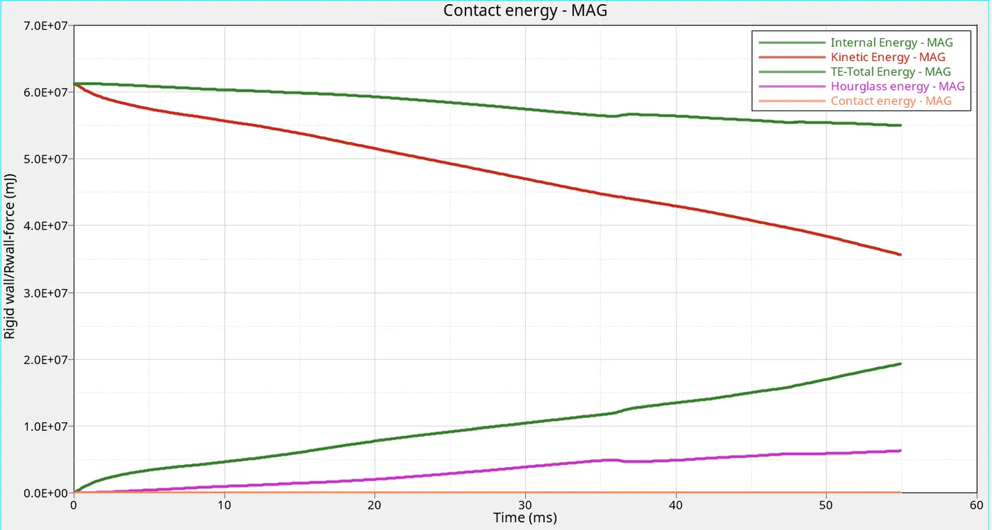
Fig 1.31: Time-History plot – Energies

From the figure 1.31, it can be seen that as the kinetic energy decreases the internal energy and the hourglass energy increases. During crash, the kinetic energy is converted to the strain energy due to the deformation of the body. Therefore as the kinetic energy decreases the internal energy increases. Since here the under-integrated shell element is used for the simulation, there is an hourglass associated with it. Due to the hourglass, the software applies the hourglass perturbation control method. This control method produces the hourglass energy which increases, as the deformation increases. For this element viscous method is used as hourglass control method, which applies only the damping to slow the speed of deformation. Therefore it will have high hourglass energy associated with this hourglass perturbation control method.

The contact force remains 0.

Case 2 – Simulation with the modified shell element properties:

In this case, the simulation is performed using the modified shell element parameter, which is best suitable for this simulation type and material of the model. The parameter chosen are as follows:

Parameters	Comment
Ishell = 24	QEPH 4 nodes Improved under-integrated shell element
Ismstr = 2	Large strain with full geometrical nonlinearities with possible small strain formulation activation in RADIOSS Engine.
Ish3n = 2	Standard 3 node shell element (C0) with modifications for large rotation
N = 5	Number of integration points set to 5 for accuracy bending.
Ithick = 1	Thickness change is taken into the account
Iplas = 1	Iterative projection with three newton iterations method for plasticity calculation

Table 2.1: Shell element Parameters

• Import the given starter input deck file of the Radioss. The file can be imported using the “Import Solver Deck” from the “File” menu or using the shortcut icon in the toolbar. Choose the file type as Radioss and select the required file name.

• The starter input has all the model information including the shell element property. For this simulation the shell element properties in the solver input deck are changed to the required values mentioned in the table 2.1.

  

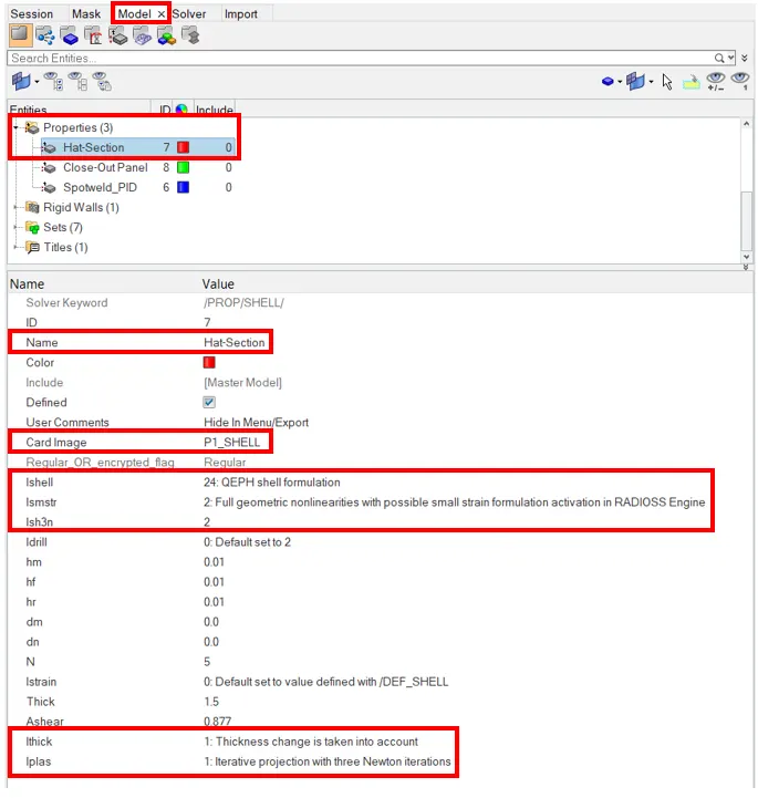
  Fig 2.1: Shell element property of hat section

  

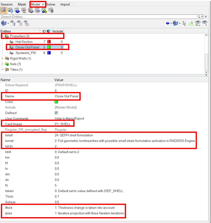
  Fig 2.2: Shell element property of close-out panel

  The important properties of the shell elements are as follows:

  Ishell: For this simulation Ishell of 24 is selected. It represents the QEPH, which is an improved under-integrated element with physical hourglass stabilization. The element of QEPH is a best compromise between the cost and the quality. The QEPH elements give accurate results during loading and unloading despite having the hourglass effect. The physical stabilization hourglass control method is used for this element.

  Ish3n: For this simulation, the Ish3n of 2, which is a standard triangle (C0) with modifications for large rotation, is used.

  Ismstr: For this simulation Ismstr of 2, which represents the large strain formulation with full geometrical nonlinearities with possible small strain formulation activation in RADIOSS Engine, is used.

  N: 5 number of integration points through the thickness are used.

  Iplas: Iplas of 1, which represents the iterative projection with three newton iterations for the calculation in plastic region, is used.

  Ithick: Ithick of 1 (thickness change is taken into account) is used.

• Repeat the steps III to X from the case 1 are performed for this case.

• The mass and the energy error occurred during this simulation is checked from the output file.

  

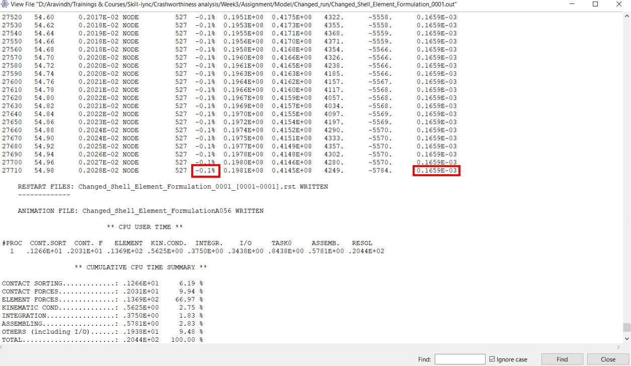
  Fig 2.3: Energy and mass error

  The energy error of -0.1% and the mass error of 0.1659E-03% is within the acceptable limit. The energy error in this case is better than the previous case error (-10.3%). The reason is due to the element type and the hourglass perturbation control method. This is the improved under-integrated element, therefore the computation is much more accurate, which leads to only small error in the result. The stiffness method is used as hourglass perturbation control method, where the method changes the stiffness to control the hourglass. Since it makes the changes in the material lever, the resultant hourglass energy during this simulation is very less.

Results from Case2:

The same results as of previous case are considered here.

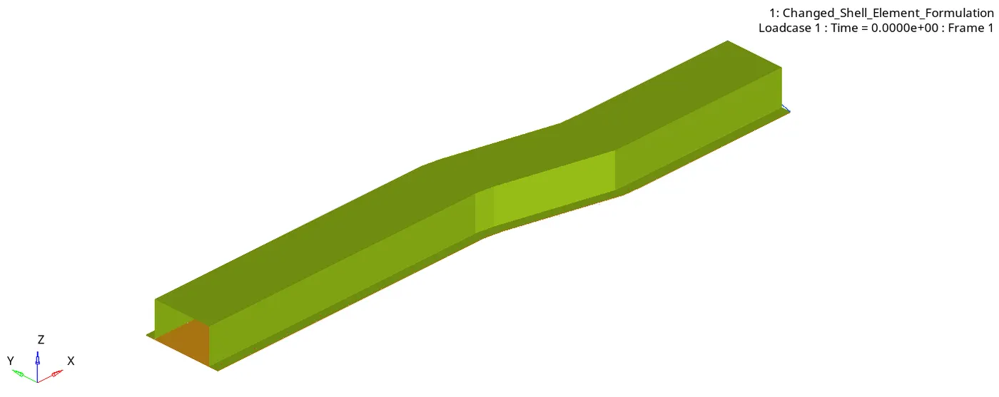
Fig 2.4: Animation of the deformation

The deformation in this case is more accurate than the previous case. The end section of the rail is experiencing small deformation till the elements at the front is completely deformed. Only after the front elements are deformed, the end elements starts deforming and reaches the maximum deformation at the end of the simulation.

The contours of the Von-Mises and plastic strain tensors are viewed to get more understanding of the behavior.

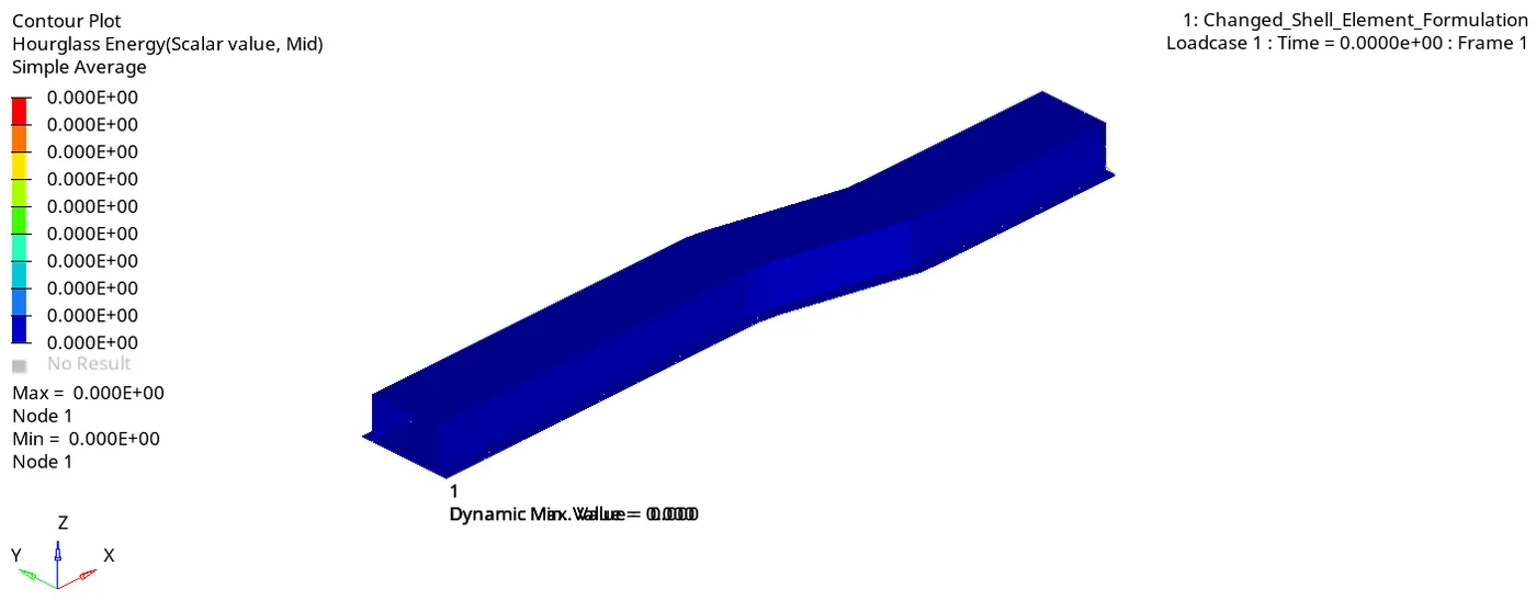
Fig 2.5: Animation of the hourglass energy

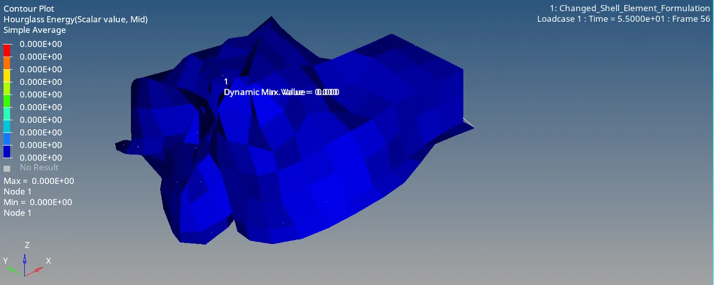
Fig 2.6: Hourglass energy at t = 55ms

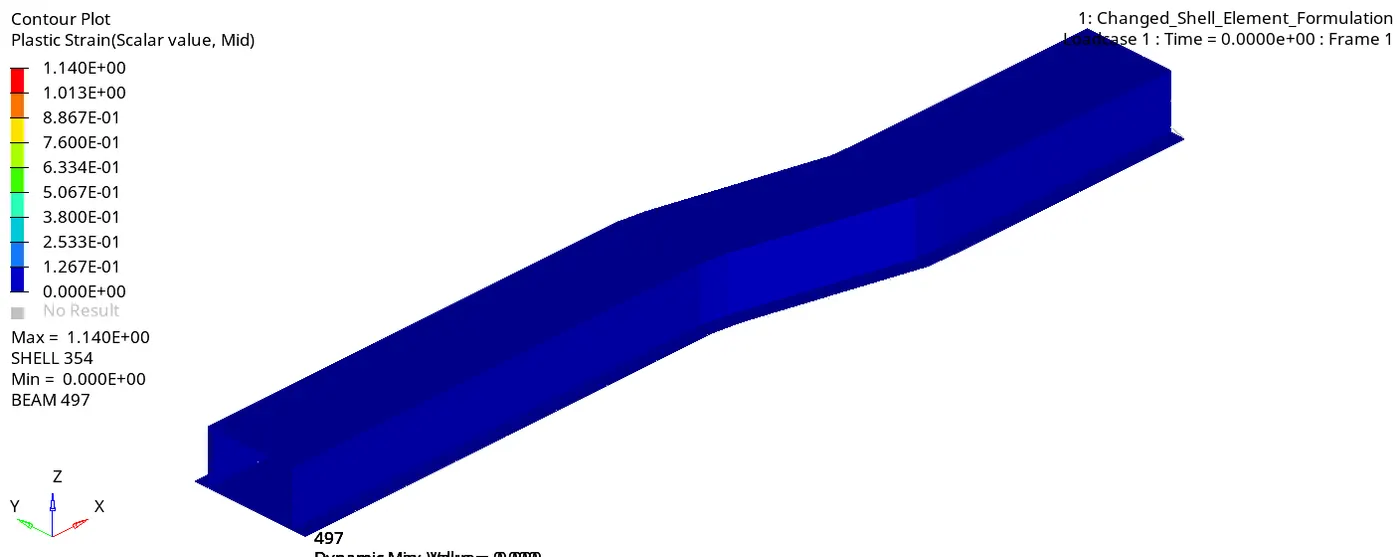
Fig 2.7: Animation of the plastic strain

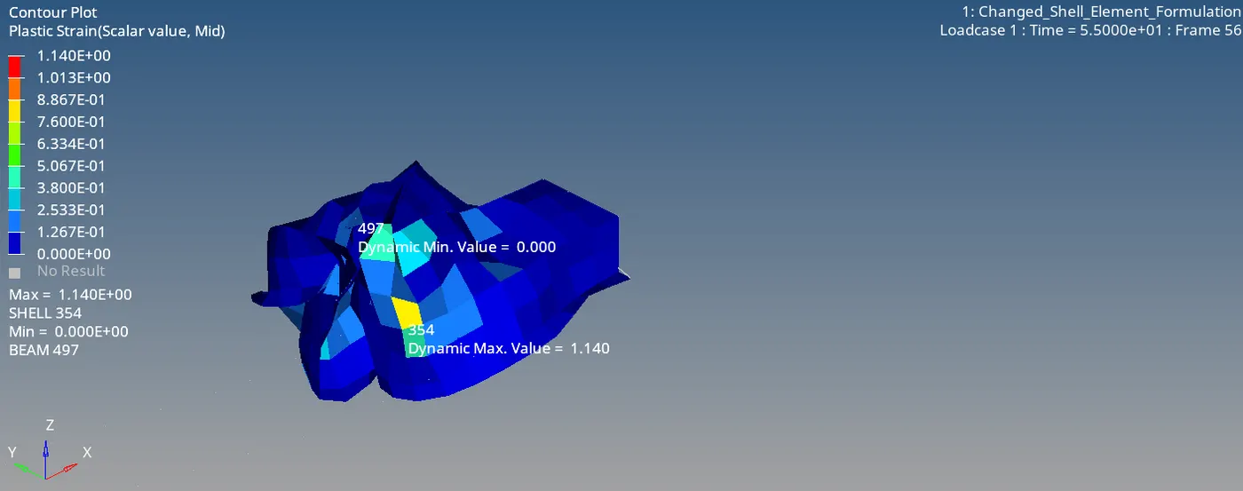
Fig 2.8: Plastic strain at t = 55ms

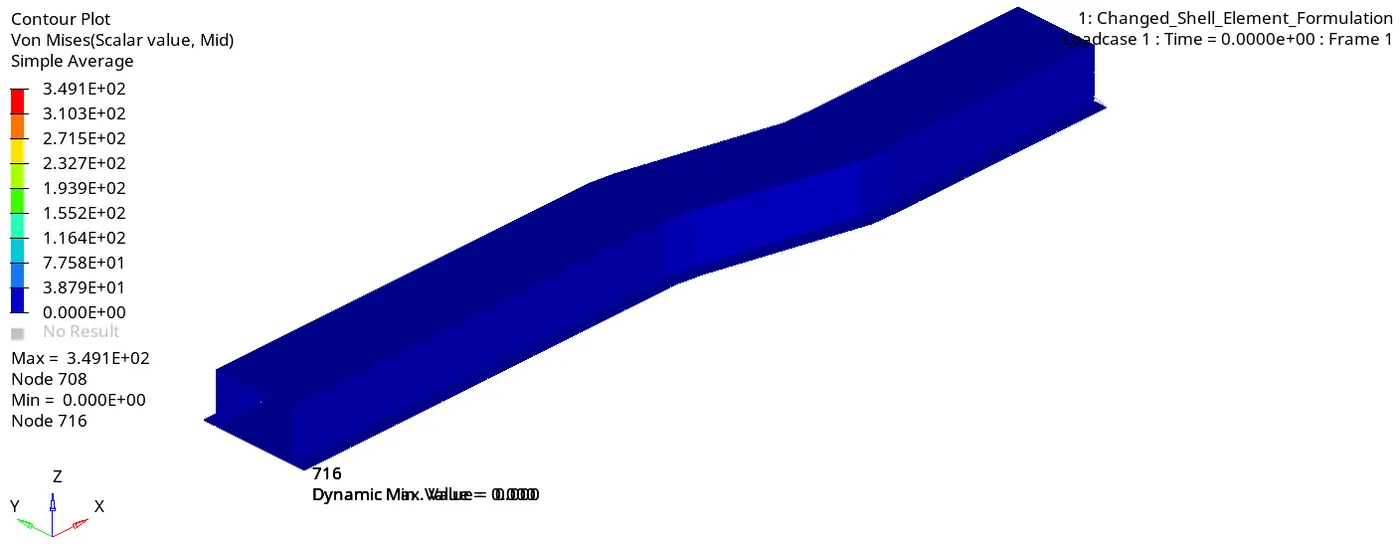
Fig 2.9: Animation of the von-mises stress

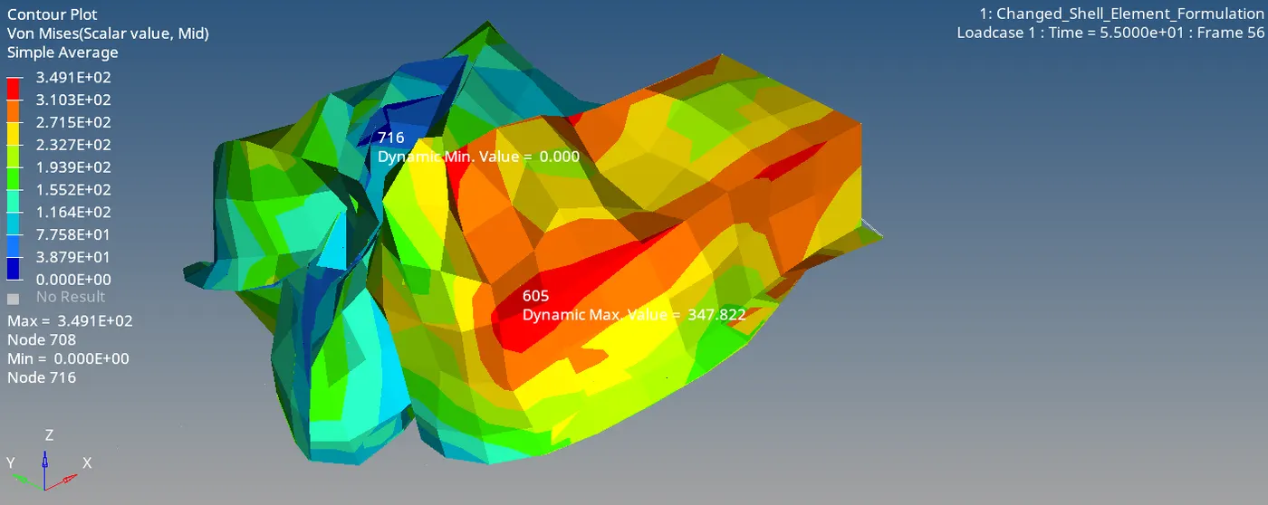
Fig 2.10: Von-mises stress at t = 55ms

The time-history plot of rigid wall forces such as total resultant force, tangential and normal resultant forces and the energies such as internal, kinetic, contact and the hourglass energy are plotted.

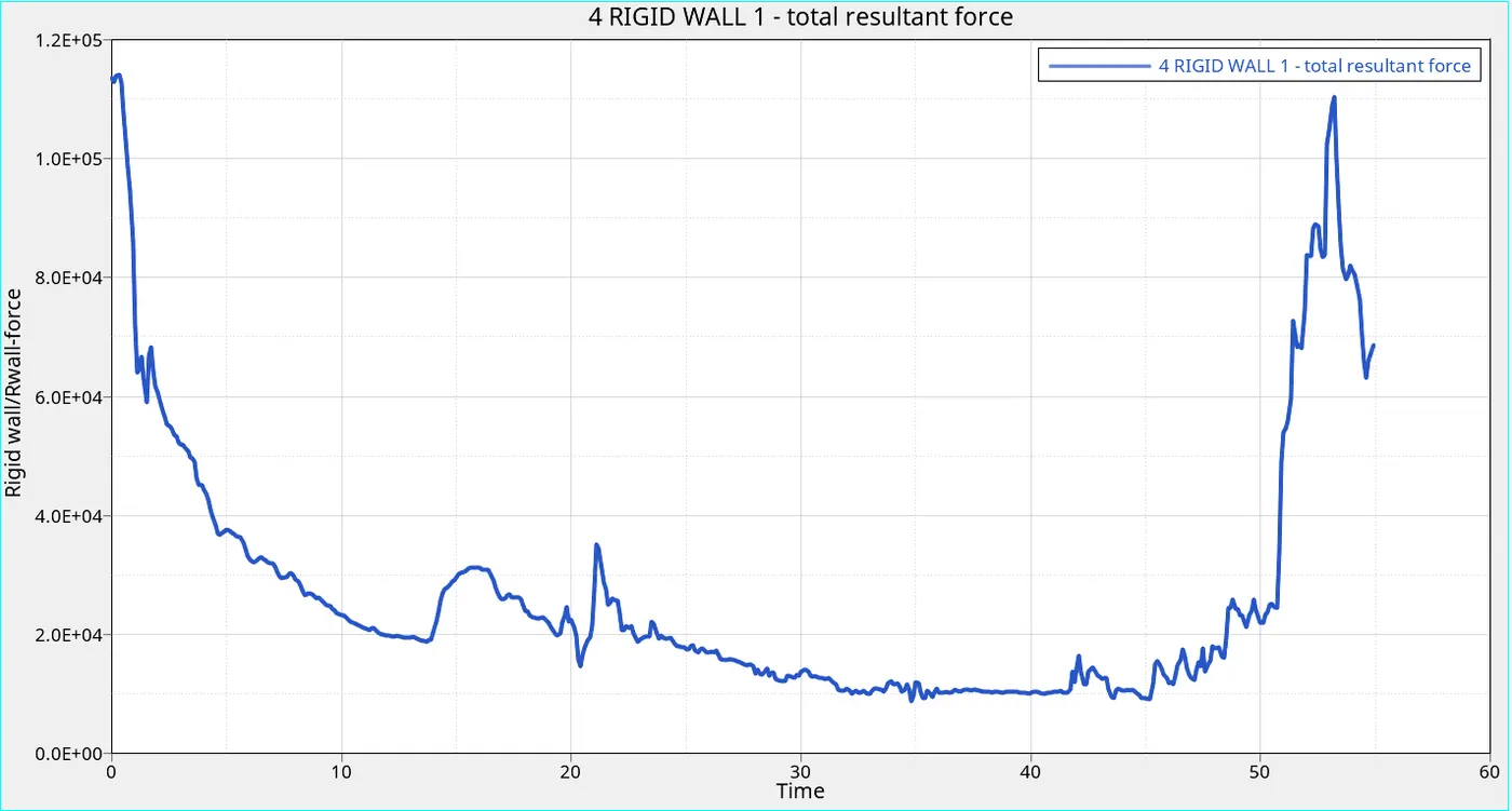
Fig 2.11: Rigid wall force – total resultant force

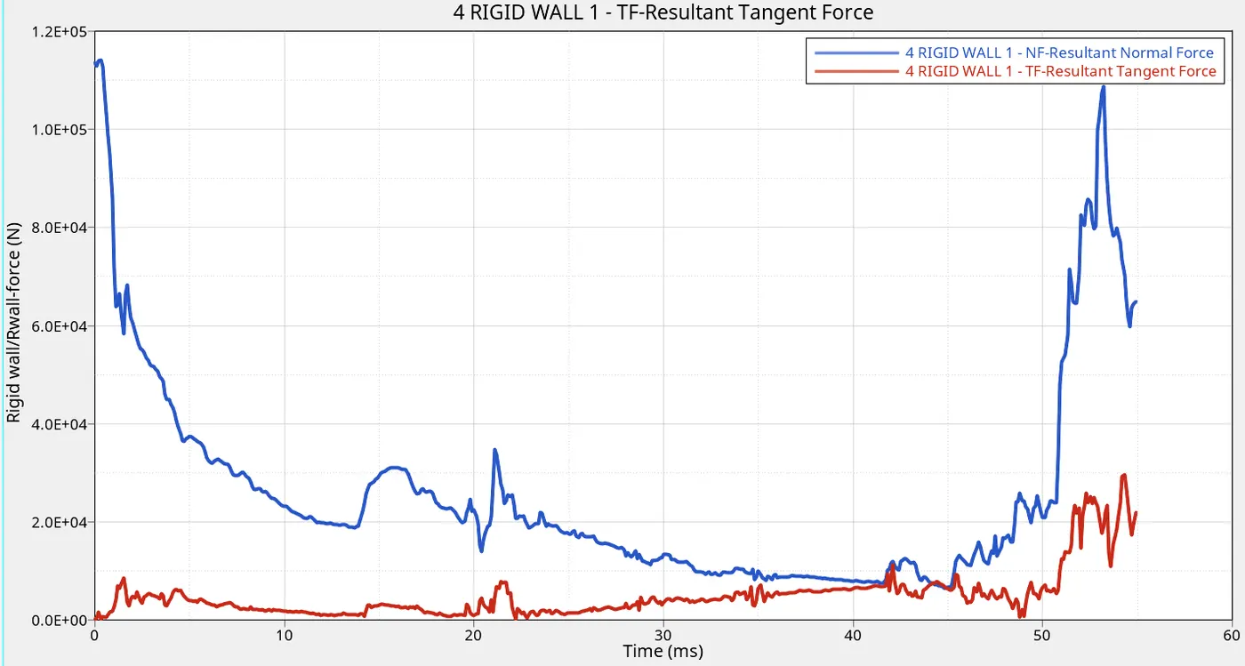
Fig 2.12: Rigid wall force – normal and tangential resultant force

From the figure 2.11, it can be seen that the total resultant rigid wall force decreases initially, then starts increasing, reaches almost the initial peak value and then decreases again. The reason can be found in figure 2.12. In this figure, it can be seen that the resultant normal force decreases initially and the tangential force remains almost same in that time period. Then normal resultant force decreases and the tangential force increases, thereby decreasing the total resultant rigid wall force. At the end the normal force and the tangential force increases, at which the total resultant forces reaches the peak. Then the normal force and the tangential force decreases, thereby reducing the total resultant force along with it.

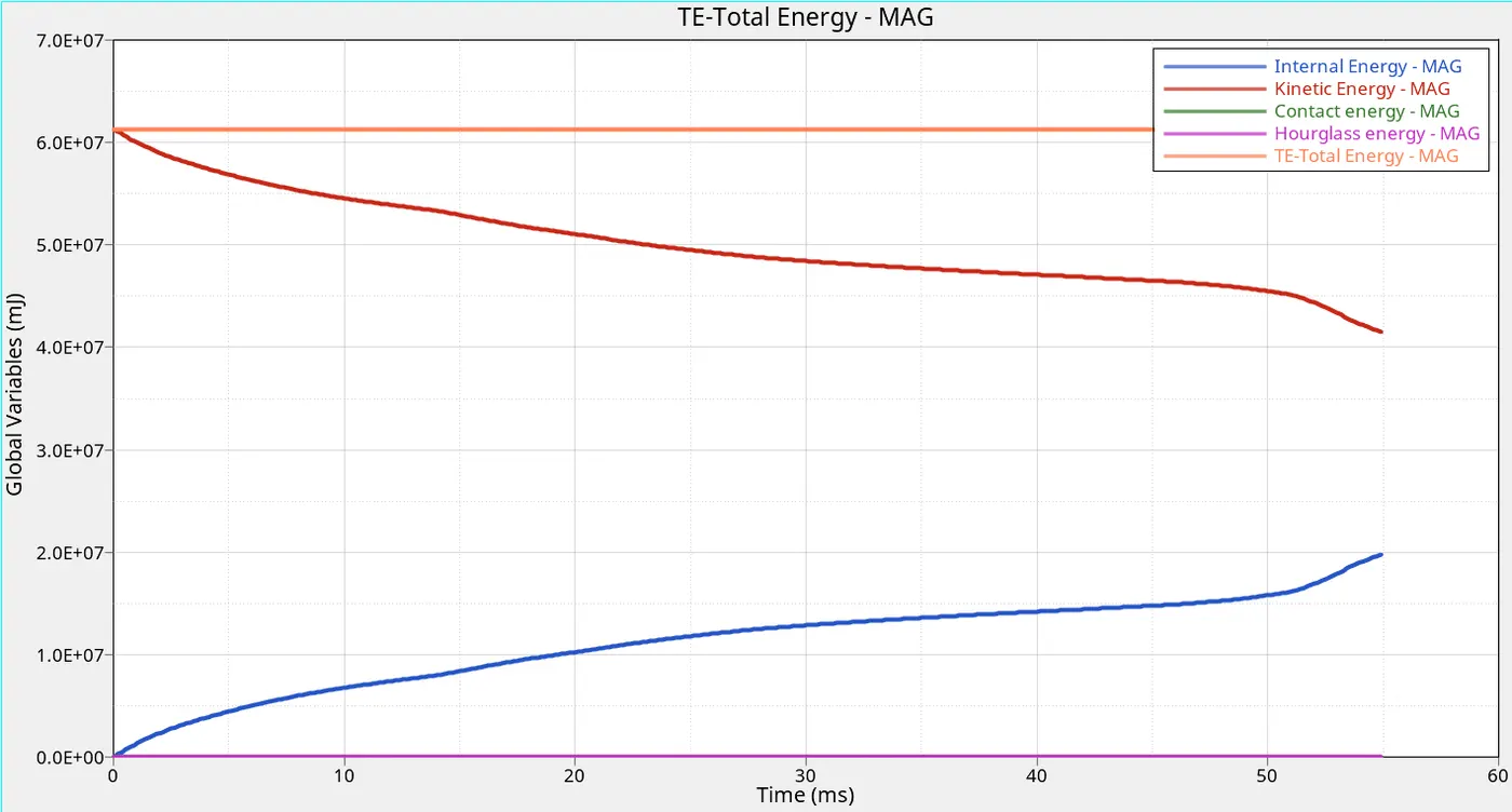
Fig 2.13: Time-History plot – Energies

From the figure 2.13, it can be seen that as the kinetic energy decreases the internal energy increases. During crash, the kinetic energy is converted to the strain energy due to the deformation of the body. Therefore as the kinetic energy decreases the internal energy increases. Since here the improved under-integrated shell element is used for the simulation, there is no hourglass associated with it. Due to the hourglass, the software applies the hourglass perturbation control method.

The contact force and the hourglass force remains 0.

Result Comparison:

The results from both the cases are compared with each other.

Deformation:

Fig 3.1: Deformation – case 1

Fig 3.2: Deformation – case 2

The deformation from the first case is bit unrealistic. The elements at the opposite side of the impact has extensive amount of deformation. The elements at that experiences high deformation and then only at the end of the simulation, the elements in the front undergo high deformation and the reason is also only due to the self-contact of the rail at the end of the simulation. This defies the physics of energy transfer. The kinetic energy will travel from the point of impact to the opposite side. Therefore, the elements at the impact region must undergo the extensive deformation initially to absorb the kinetic energy and only then the due to remaining high kinetic energy, the end elements undergo high deformation to absorb that remaining kinetic energy.

The deformation in this case is more accurate than the previous case. The end section of the rail is experiencing small deformation till the elements at the front is completely deformed. Only after the front elements are deformed, the end elements starts deforming and reaches the maximum deformation at the end of the simulation.

Hourglass energy:

Fig 3.3: Hourglass energy – case 1

Fig 3.4: Hourglass energy – case 2

Since for case 1 the under-integrated shell element is used for the simulation, there is an hourglass associated with it. Due to the hourglass, the software applies the hourglass perturbation control method. This control method produces the hourglass energy which increases, as the deformation increases. For this element viscous method is used as hourglass control method, which applies only the damping to slow the speed of deformation. Therefore it will have high hourglass energy associated with this hourglass perturbation control method.

Whereas for case 2, the improved under-integrated shell element is used for the simulation. This element giver accurate computational results. Even though this element has the hourglass associated with it generally, the hourglass perturbation control method is stiffness method. Since, it changes the stiffness at the element level, the resultant hourglass energy is very small. But in this simulation, there is no hourglass energy.

Plastic Strain:

Fig 3.5: Plastic strain – case 1

Fig 3.6: Plastic strain – case 2

Due to the hourglass deformation associated with case 1, the plastic strain is less. Since hourglass modes are zero energy modes, the stress and strains are zero for these elements. Therefore, due to the hourglass effect on few elements, the strain for those elements are zero, which led to less strain value. The maximum strain value is 0.5572 for case 1 and 0.6386 for case 2.

Von-Mises Strain:

Fig 3.7: Von-mises stress – case 1

Fig 3.8: Von-mises stress – case 2

The variation of the stress throughout the simulation time can be viewed exactly in case 2 than in case 1. The stress value in the middle section from case2 is much more than case1, since case 1 has hourglass associated at that section. The maximum strain value is 349.9 MPa for case 1 and 349.1 MPa for case 2.

Rigid wall forces:

Fig 3.9: Total resultant rigid wall forces – case 1

Fig 3.10: Total resultant rigid wall forces – case 2

From the figure 3.9, it can be seen that the total resultant rigid wall force decreases initially and then starts increasing. The spikes in the graph denotes the elements contacting the wall. The force reaches the value of 0 N at 6 ms, indicating no elements are contacting the wall. Then the force again starts increasing.

From the figure 3.10, it can be seen that the total resultant rigid wall force of case 2 decreases initially, then starts increasing, reaches almost the initial peak value and then decreases again. The force reaches peak at almost 53 ms, denoting that many new elements are contacting the rigid wall. After that the force starts decreasing again.

The final force at the end of the simulation is high for case 2 than case 1, since the deformation behavior of the case 2 is much more accurate and realistic than case 1, thereby many elements came into contact with the wall in case 2 simulation at 53 ms, when compared to the number of elements at 53 ms in case 1.

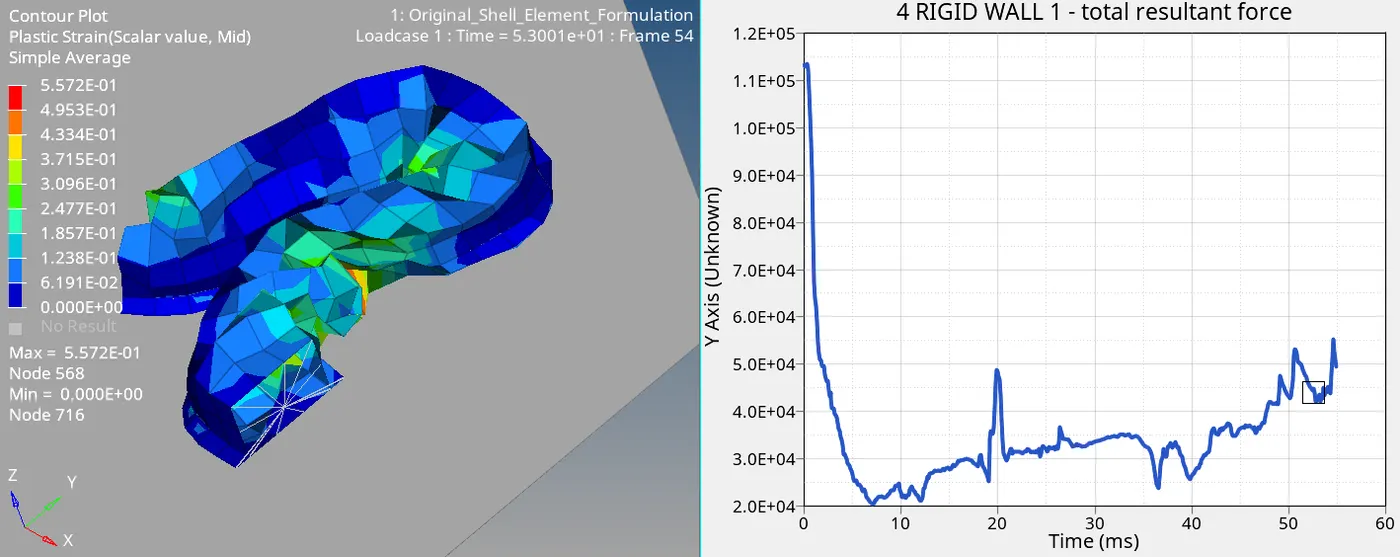
Fig 3.11: Elements contact with wall at 53 ms – case 1

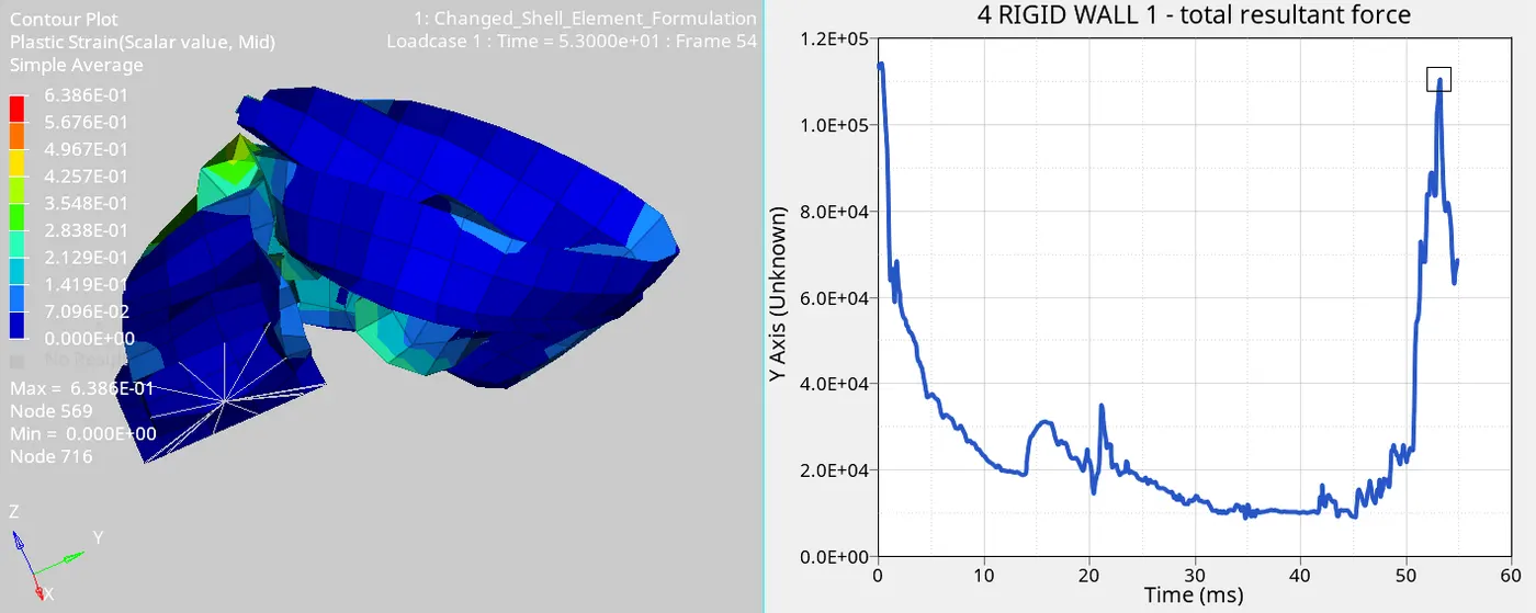
Fig 3.12: Elements contact with wall at 53 ms – case 2

Energies:

Fig 3.13: Time-History plot – Energies – case 1

Fig 3.14: Time-History plot – Energies – case 2

From the figure 3.13, it can be seen that as the kinetic energy decreases the internal energy and the hourglass energy increases. During crash, the kinetic energy is converted to the strain energy due to the deformation of the body. Therefore as the kinetic energy decreases the internal energy increases. Since here the under-integrated shell element is used for the simulation, there is an hourglass associated with it. Due to the hourglass, the software applies the hourglass perturbation control method. This control method produces the hourglass energy which increases, as the deformation increases. For this element viscous method is used as hourglass control method, which applies only the damping to slow the speed of deformation. Therefore it will have high hourglass energy associated with this hourglass perturbation control method.

From the figure 3.14, it can be seen that as the kinetic energy decreases the internal energy increases. The improved under-integrated shell element is used for the simulation. This element giver accurate computational results. Even though this element has the hourglass associated with it generally, the hourglass perturbation control method is stiffness method. Since, it changes the stiffness at the element level, the resultant hourglass energy is very small. But in this simulation, there is no hourglass energy.

The total energy remains constant for case 2, since the energy is well balanced and the energy error is only -0.1%, whereas for case 2, the total energy also reduces due to the high energy error (-10.3%) in the system.

Conclusion:

Thus the effects of various shell parameters on the simulation results are studied in detailed and the best combination of shell element parameters are determined, which will be used in the future simulations.

The simulation using the recommended shell element property of Ishell of 24, Ish3n of 2, Ismstr of 2, N = 5, Iplas of 1 and Ithick of 1 gives the more accurate result and are the best combination of shell element parameters for the crash analysis.

Using these parameters the energy error was almost eliminated, due to the zero hourglass energy, which resulted in better energy balance.

Hourglass Energy:

Hourglass modes are zero energy modes. Each element velocity vector can be seen in 4D space and decomposed along 4 physical vectors: rigid body translation, tension-compression, simple shear and hourglasssing (or in-plane bending). The last vector hourglass leads to zero strain value at the element center. And when the under-integrated elements are used, where there is only one gauss point and which lies at the element center, will lead to interpolating the zero strain value along the entire element, which give rise to zero energy. Since the element deforms along the region where the energy is minimum, this zero energy causes extreme deformation. These deformation will be in the shape of hourglass, therefore the name hourglass effect.

These hourglass modes has to be suppressed. The hourglass effect can be avoided by using fully integrated element. But the simulation time will be high. Instead the under-integrated elemnts can be used along with the hourglass perturbation control methods.

Hourglass Perturbation Control Method:

1. Perturbation (Viscous) method I_shell = 1,2,3 or 4 (Q4):

   In the viscous method, when the hourglass deformation occurs, a damping is applied. And because of this damping, the deformation will be stabilized. The damping will control the speed at which the deformation is happening. The damping is only going to oppose the velocity not the force. By applying the damping a force is generated, which affects only the speed of the deformation. This control of hourglass perturbation creates energy called hourglass energy.

   The hourglass energy is the mathematically created energy. It does not exist in nature. It is neither kinetic nor internal energy. Hourglass energy is the loss of both the energy.

2. Perturbation method I_shell = 24 (QEPH) = stiffness method:

   In this case, the stiffness is artificially added to the element. To add the stiffness, it is going to affect the material properties directly. The stiffness is added at the material level. Since, it is happening at the material level, this method will have larger effect on the component.

   Since it is applied at the material level, it is getting added even before the hourglass deformation, thereby preventing the creation of hourglass modes, unlike viscous method, which applies damping after the hourglass deformation resulting in more hourglass energy. Therefore for stiffness method, only less amount of hourglass energy is required for controlling the hourglass effect.

   The stiffness method is mostly used hourglass control method in the automotive field.

Ideally for a simulation, the numerically created hourglass energy must not exceed 5% of the total energy of the system, since it is artificially created energy, when it exceed 5%, it gives inaccurate results in the physical sense.

Bibliography:

Altair Engineering, Inc. (2019), Altair Radioss Help, https://2019.help.altair.com/2019/rad/topics/solvers/rad/faq_rad_results_checking_r.htmzoom_highlightsub=energy+error