Radioss Engine File Editing and 3D Meshing using HyperMesh

Radioss Engine File Editing and 3D Meshing using HyperMesh:

Objective:

The objectives of this assignments are

1. Edit the given engine input file
   1. Calculate the speed of the sound in steel
   2. Calculate the time taken by the sound wave to propagate through the steel rail of 1000 mm
   3. Edit the termination time in /RUN card of the engine file
   4. Edit the frequency of the animation output such that there are 20 steps, by editing it in /ANIM/DT card.
2. Perform the 3D meshing of the housing and arm bracket within the required element quality.

Editing the RADIOSS Engine File:

Tasks:

The main task of this section is to edit the engine input file created by Radioss. The parts to be edited in the Radioss engine file are as follows:

• Edit the termination time in the /RUN card by calculating the time taken for sound to travel through the length of the rail.
• Change the frequency of the animation output by editing /ANIM/DT card
• Change /Print -10

Given:

For the problem, the input solver deck “FIRST_RUN_0000.rad” and the engine file “FIRST_RUN_0001.rad are given. The length of the rail is 1000 mm.

Input Solver Deck:

The input solver deck is file generated by the Radioss or by the user, which contain the model information such as material properties, material law, nodes, elements along with their nodes, loading conditions etc. It is in the format similar to that of text file. Therefore the user can edit it easily without going to HyperWorks again. Each detail of the models are specified according to a specific format which contains keywords for each sections / cards and format for entering the values in it. The file name of it will be in the format “filename_0000.rad”.

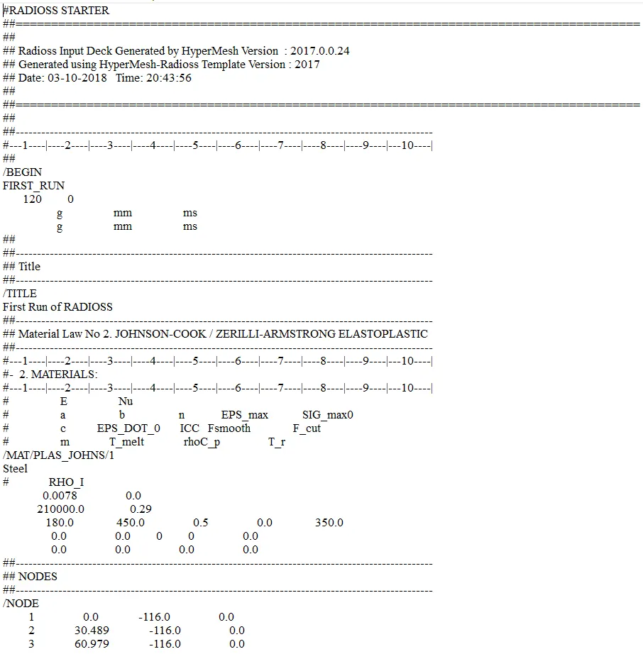
Fig 1.1: Input solver deck

The detailed explanation of each cards of the input solver deck are represented by the following images.

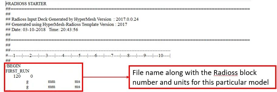
Fig 1.2: Input solver deck starting

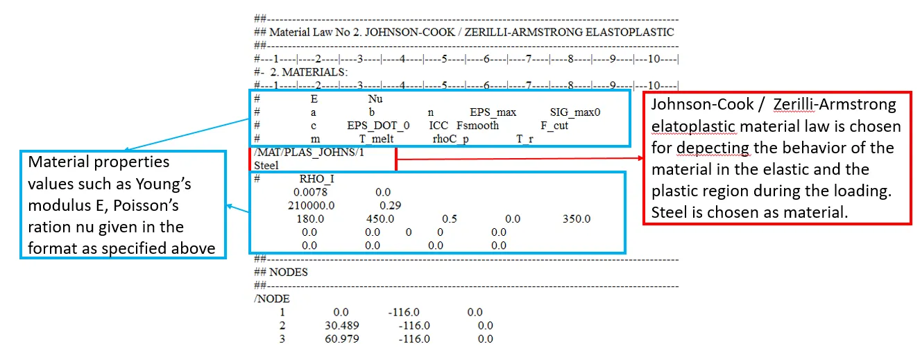
Fig 1.3: Material properties

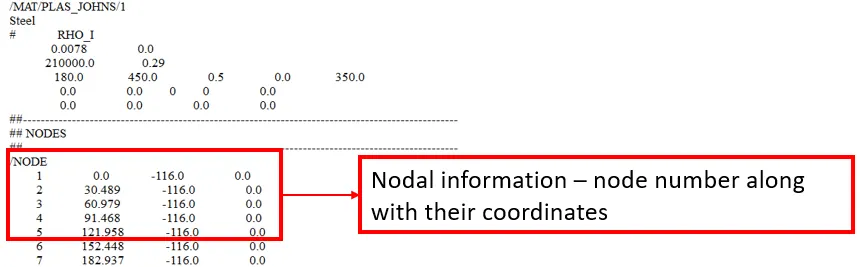
Fig 1.4: Nodal information

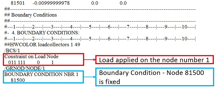
Fig 1.5: Boundary conditions

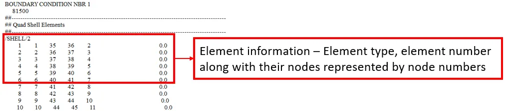
Fig 1.6: Element information

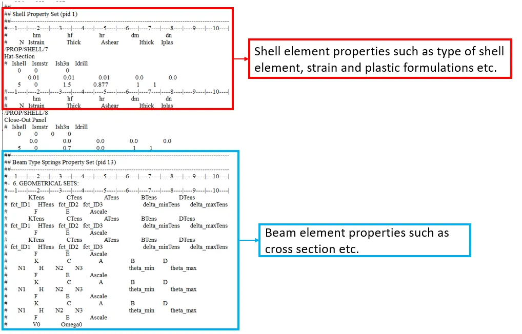
Fig 1.7: Element properties

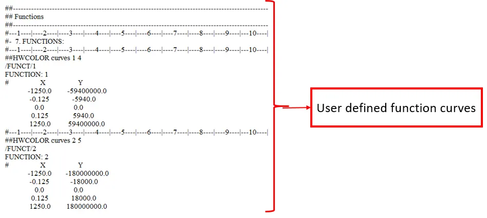
Fig 1.8: User-defined functions

For crash analysis, the initial velocity has to be specified, which represents the velocity of the vehicle. The initial velocity chosen is based on the type of crash analysis such as front or side or rear crash analysis and the regulation such as EURO-NCAP or US-NCAP.

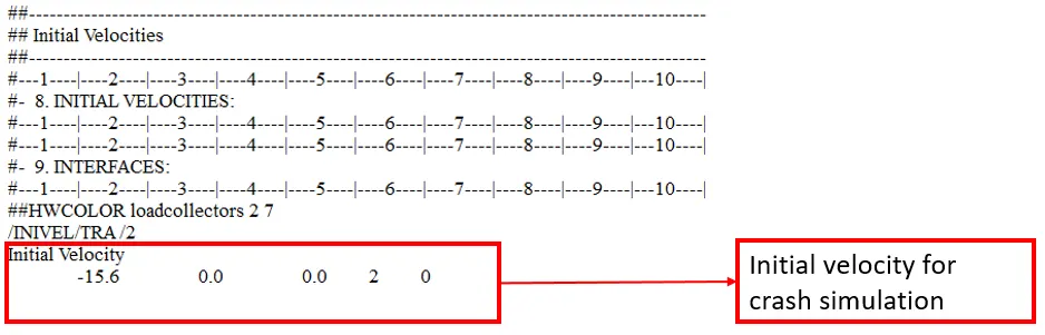
Fig 1.9: Initial velocity for crash

Contact / Interface plays a major role in the crash analysis. The contact between the surfaces or node and surface induces non-linearity which has to be captured perfectly for the accurate result. Contact energy contributes to a lot during the deformation after the crash. Due to the interface, there is a friction and this friction absorbs some of the kinetic energy of the vehicle. There are different type of contact formulations and it varies according to the silver used. One of the most common type is Node-Segment-Interface type. It uses a master slave concept. In many solvers it is a one way contact, in which software check whether the slave node penetrates the master surface. Other type is two way contact, in which the software check for both the slave and master segments for penetration. The interface has to be defined such that there are no initial penetration. The penetration leads to the numerical creation of the energy during the crash simulation, even though it is not possible in the physical terms. This numerically created energy leads to wrong results. Thus the penetration has to be avoided in the modelling.

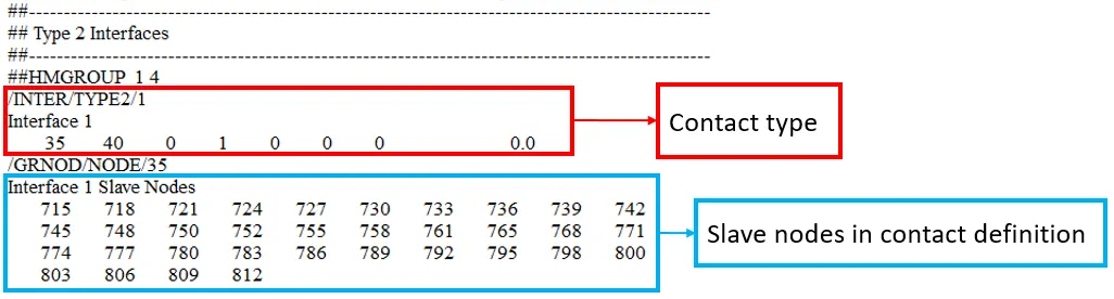
Fig 1.10: Contact type and slave nodes information

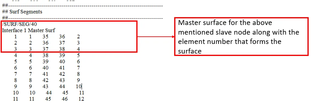
Fig 1.11: Master surface information

Since here the rail is crashed against the wall, which is rigid, it has be defined as rigid. Rigid body does not undergo any deformation. For rigid body the Poisson’s ratio is 0.5.

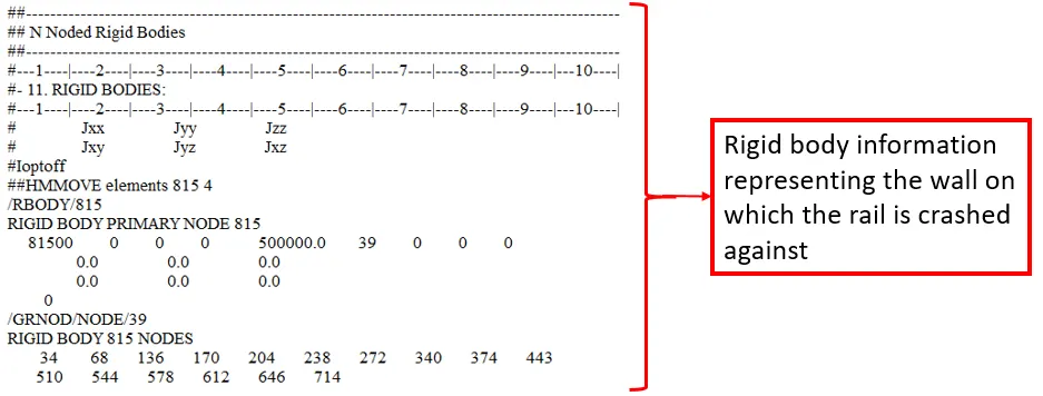
Fig 1.12: Rigid body – wall

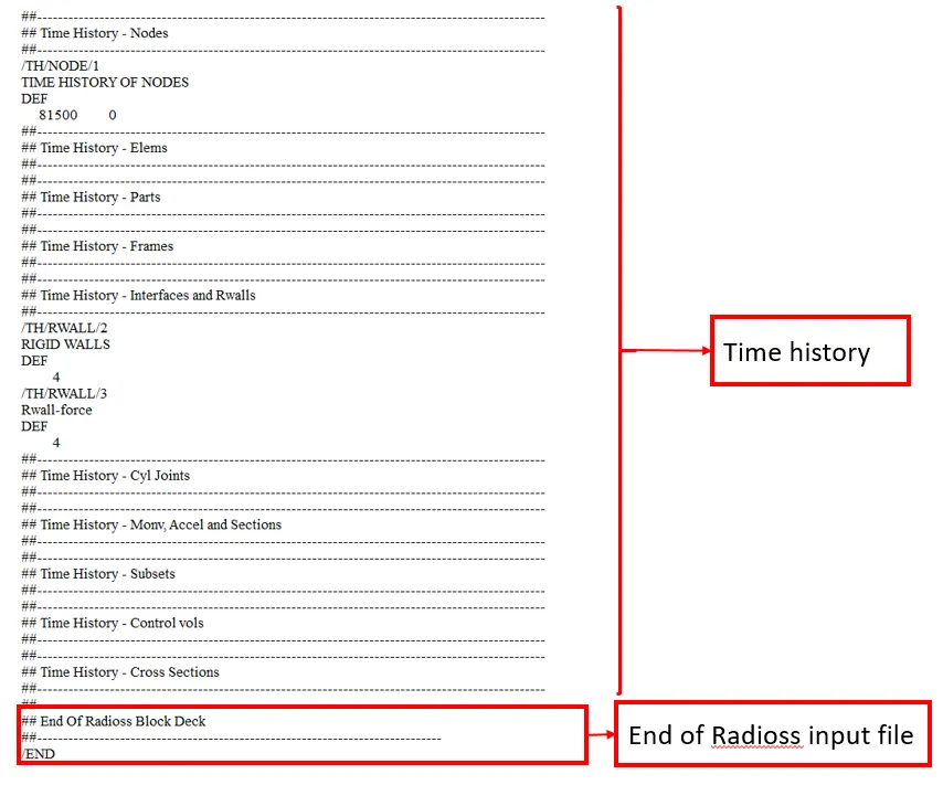
Fig 1.13: Time History and End of solver deck

Engine Input FIle:

The engine input file consists of run parameters such as time step and termination time and also post-processing parameters such as required animations at the end of simulation such as stress, displacement and also time-history plots for energy etc. The file name of it will be in the format “filename_0001.rad”.

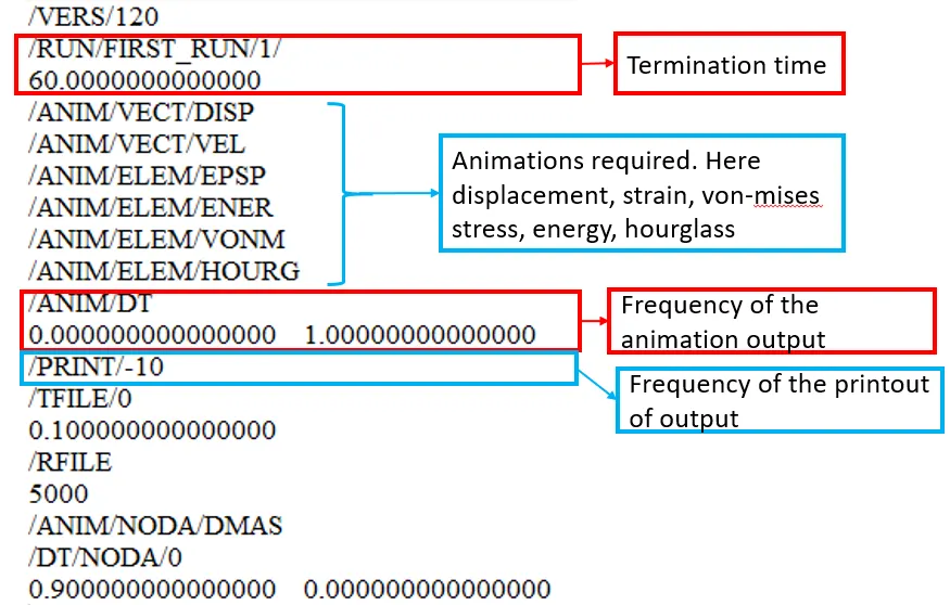
Fig 1.14: Engine Input File

Usage of Starter Input Deck:

The user can open and edit both the starter input deck and the engine input file as required. But if the user is not sure about the position of change such as nodal changes, the user can import the starter input deck into the Radioss and perform the change. The file can be imported using the “Import Solver Deck” from the “File” menu or using the shortcut icon in the toolbar.

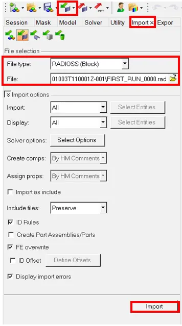
Fig 1.15: Import solver deck

Choose the file type as Radioss and select the required file name.

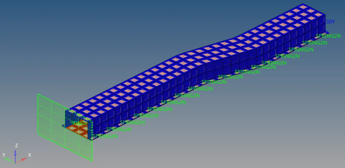
Fig 1.16: Model of FIRST_RUN_0000.rad

Calculation of the time step:

Crash simulation is a large deformation problem. Therefore it is an explicit analysis. The explicit analysis gives the acceleration at nth time step, from which the velocity at time step and acceleration at n+1 time step are calculated.

Unlike the implicit analysis, the explicit analysis does not iterate to equilibrium for each time step. Therefore it is not unconditionally accurate. The accuracy depends on the time step. Larger time step like implicit analysis cannot be used for the explicit analysis. The time step chosen for the explicit analysis must be less than the courant time.

Courant time step is the time required for the sound wave to pass through one element. There it is dependent on the speed of the sound and the element length.

`Deltat_c < frac{l_c}{C}`

Where, t_c – Courant time step

l_c – smallest element length

C - Speed of the sound on that material.

The speed of the sound in turn depends on the properties of the material such as young’s modulus, density.

`C = sqrt (E/rho)`

Where, E – Young’s modulus

`rho` – Density

The material properties of the steel is taken from the starter input deck.

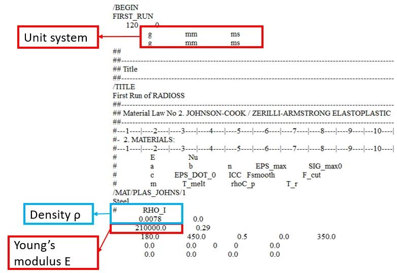
Fig 1.17: Young’s modulus and density values

From the figure 1.17, the values of the Young's modulus and the density of the material are taken.

E = 210000.0 MPa

ρ = 0.0078 K Kg/l

The unit systems are consistent with the Radioss unit system.

`C = 5188.7452 frac{mm}{ms}`

The speed of the sound in steel is 5188.7452 mm/ms or 5188.7452 m/s.

The length of the rail (l_r) is 1000 mm.

The time taken for the sound wave to propagate through the length of rail

`t = frac{l_r}{C}`

`t = frac{1000}{5188.7542}`

`t = 0.1927 ms`

The time taken by sound wave to propagate through the steel rail of length 1000 mm is 0.1927 milliseconds.

20 animation steps has to be there at the output. The total time is 0.1927 ms. Therefore

`t_(fq) = frac{t}{20}`

`t_(fq) = frac{0.1927}{20}`

`t_(fq) = 0.009635`

Therefore the animation has to be captured for every

These values has to be inserted in the engine input file.

Editing Engine Input File:

There are two ways of changing the engine input file. One is editing the .rad file directly, by opening it in the text editor. The other being importing the input solver deck and editing the engine file in the Radioss itself.

Editing the .rad file directly:

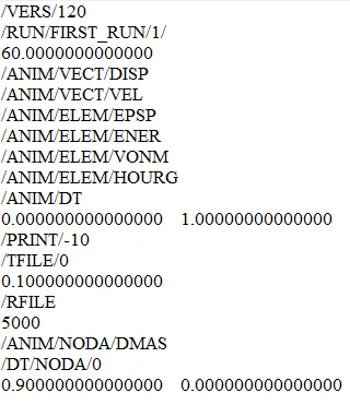
Fig 1.18: FIRST_RUN_0001.rad initial

The termination time t = 0.1927 ms. It has to be included in the /RUN card

The frequency of the animation capture t_freq = 0.009635 ms. It has to be included in the /ANIM/DT card

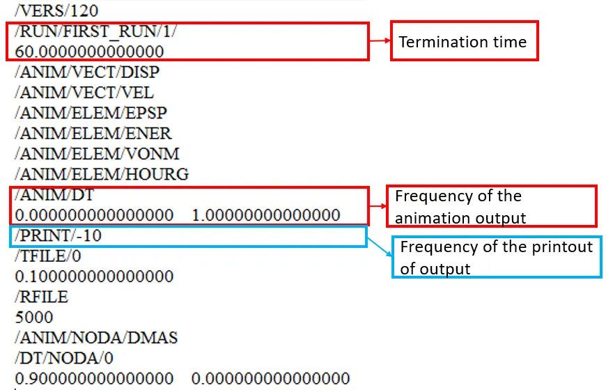
Fig 1.19: FIRST_RUN_0001.rad initial

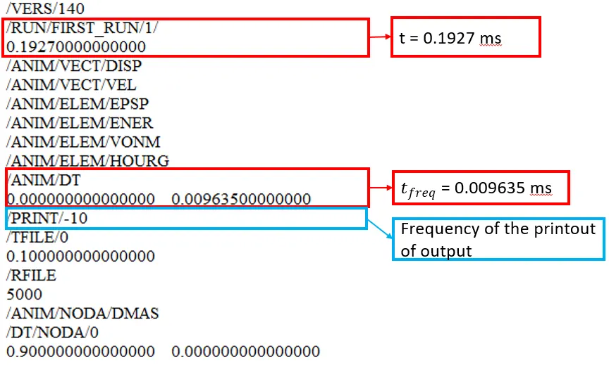
Fig 1.20: FIRST_RUN_0001.rad final

Editing the engine file through Radioss:

Import the FIRST_RUN_0000.rad using the “Import Solver Deck” option from “File” menu.

From the “View” menu activate the “Solver” deck from the “HyperMesh Browser”.

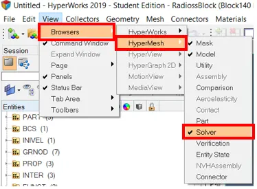
Fig 1.21: Solver deck

In the solver there is a separate drop down menu for the “Engine_Keywords”. There the user can edit the above mentioned changes.

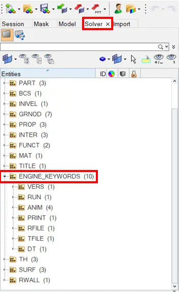
Fig 1.22: Solver deck

For editing /RUN card, go to /RUN drop-down menu and insert the new termination time in the editor.

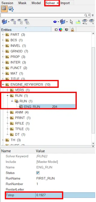
Fig 1.23: Editing /RUN card

For editing /ANIM/DT card, go to /ANIM drop-down menu and insert the new t_freq = 0.009635 ms in the /ANIM/DT editor.

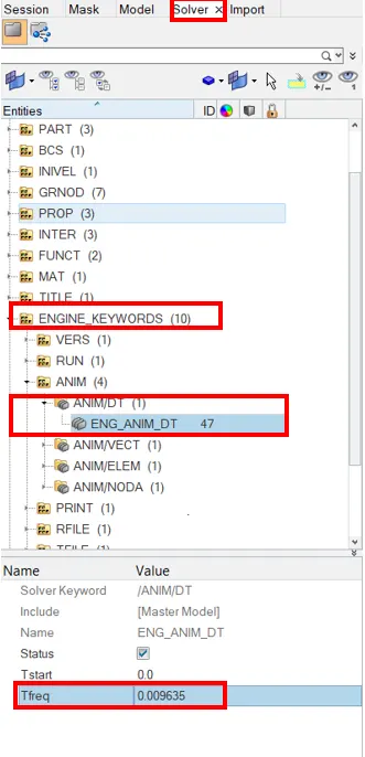
Fig 1.24: Editing /ANIM/DT card

Listing File (.out file):

Both the starter input deck and the engine input file create the listing file (.out file). The .out file can be extracted by running the problem in Radioss.

To run the model, “Radioss” option is chosen from the “Analysis” menu. The file name of the starter input deck has to be specified.

Fig 1.25: Analysis option

Fig 1.26: Run a analysis in Radioss

This run creates the listing file of starter input deck in the format of “Filename_0000.out” and the listing file of engine input deck “Filename_0001.out”. For the further simulations using this result, the software will produce the listing files of engine input deck as “Filename_0002.out”, “Filename_0003.out” and so on.

Alternatively the listing (.out) file of the starter input deck alone can be created by performing the “check” instead of “analysis” in the “run option” menu.

Fig 1.27: Check model in Radioss

Listing file of the starter input deck:

The listing (.out) file of the starter input deck contains the same model information, but it would have written according to software’s understanding of the model such as dividing the model into parts, loads etc.

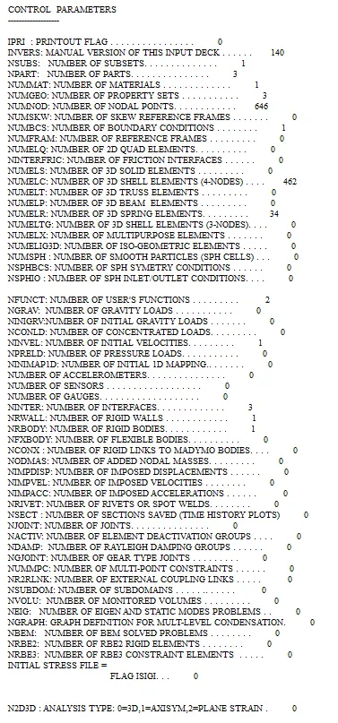
Fig 1.28: Control parameters in FIRST_RUN_0000.out

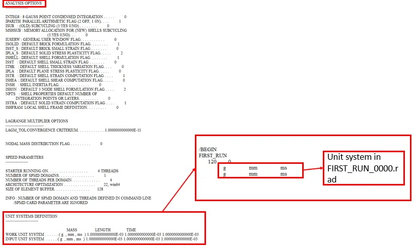
Fig 1.29: Analysis parameters and unit systems in FIRST_RUN_0000.out

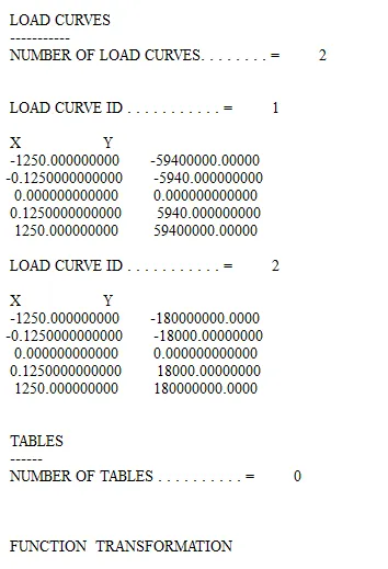
Fig 1.30: Load curves in FIRST_RUN_0000.out

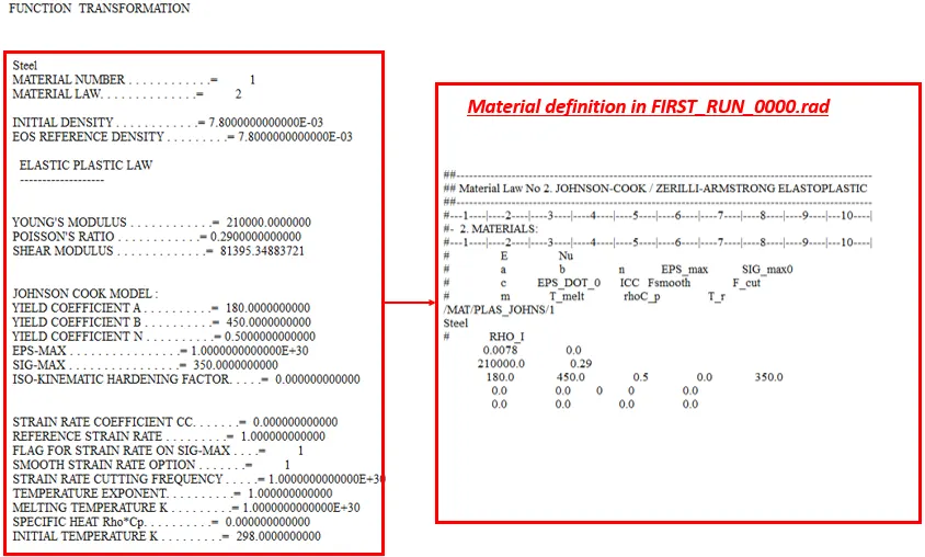
Fig 1.31: Material defintion in FIRST_RUN_0000.out vs. in FIRST_RUN _0000.rad files

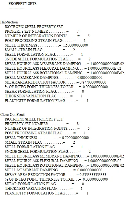
Fig 1.32: Property sets FIRST_RUN_0000.out

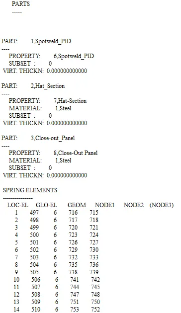
Fig 1.33: Parts along with elements and corresponding node numbers in FIRST_RUN_0000.out

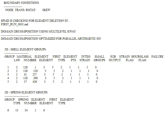
Fig 1.34: Boundary conditions in FIRST_RUN_0000.out

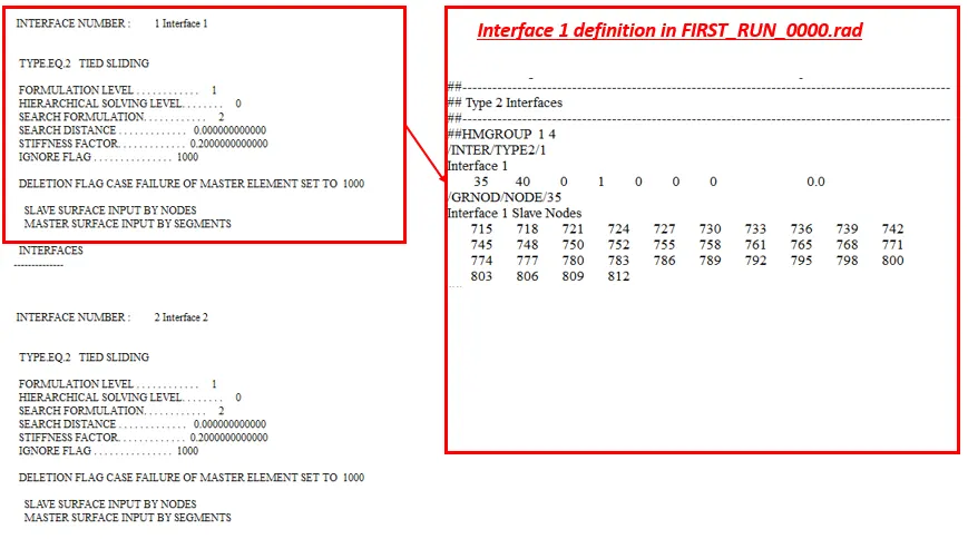
Fig 1.35: Interface defintion in FIRST_RUN_0000.out vs. in FIRST_RUN _0000.rad files

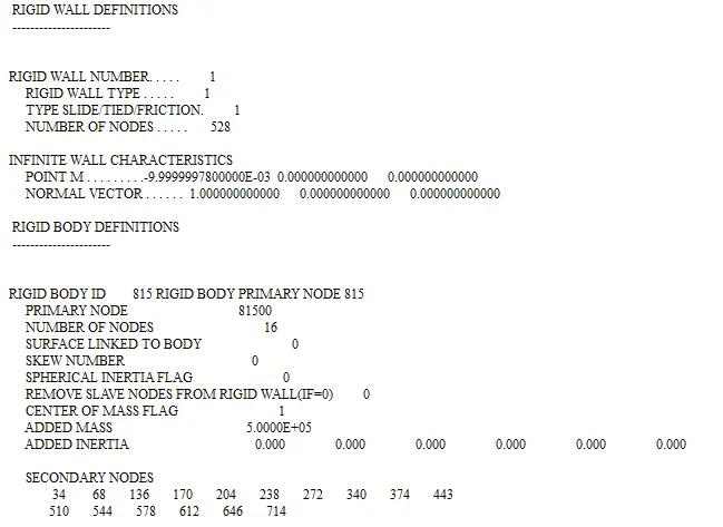
Fig 1.36: Rigid wall definition in FIRST_RUN_0000.out

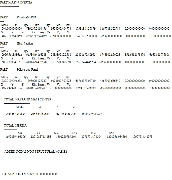
Fig 1.37: Part properties in FIRST_RUN_0000.out

From the figures 1.28 to 1.37 it can be seen that, the starter input deck file FIRST_RUN_0000.rad has been modified by the solver to its own format.

Listing file of the starter input deck:

The listing (.out) file of the engine input file contains the information of the output during and after the end of simulation such as energy balance information, time taken or completed information etc.

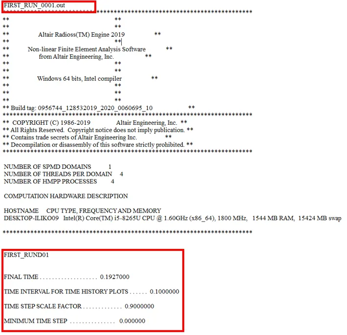
Fig 1.38: FIRST_RUN_0001.out

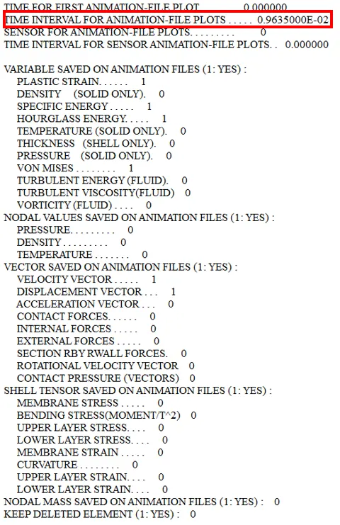
Fig 1.39: FIRST_RUN_0001.out

It can be seen from the above figures, that the changed value is being displayed in the Engine listing file (.out file). Therefore, the edited values are taken for the simulation.

The speed of the sound in steel and the time taken by the sound wave to travel through the length of the steel rail has been successfully calculated. These calculated values are given as the termination time and the frequency of the animation output in the engine input file by two different methods. The resultant listing files (.out files) of both the starter input deck and the engine input file has been obtained and given in the report.

3D Meshing - Housing:

Geometry:

This housing consists of two components: a hub and a cover.

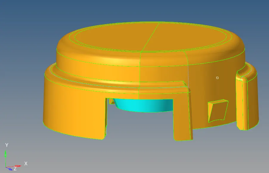
Fig 2.1: Housing

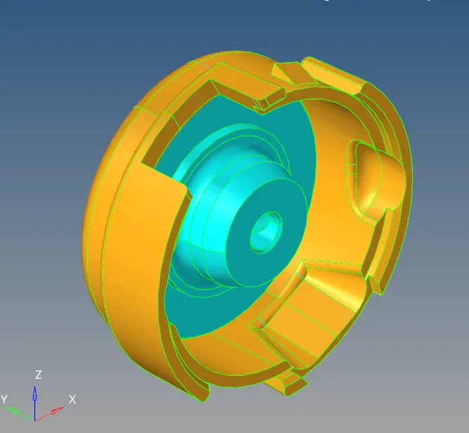
Fig 2.2: Housing with the view of both cover and hub

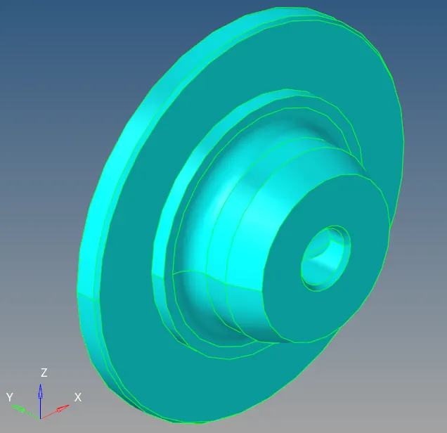
Fig 2.3: Hub

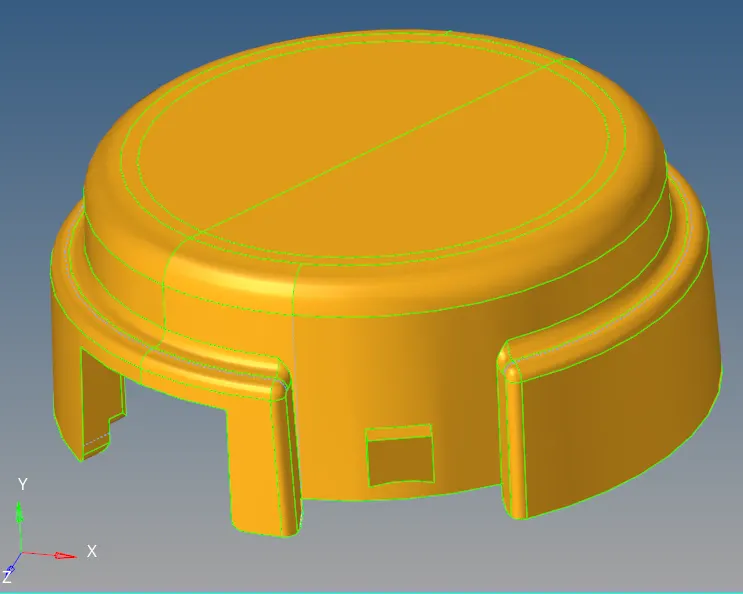
Fig 2.4: Cover

Meshing:

Since it has two components, each components are meshed independently. And since it is a solid components, solid elements are used for meshing instead of extracting the mid-surface and using shell elements on it to represent the components.

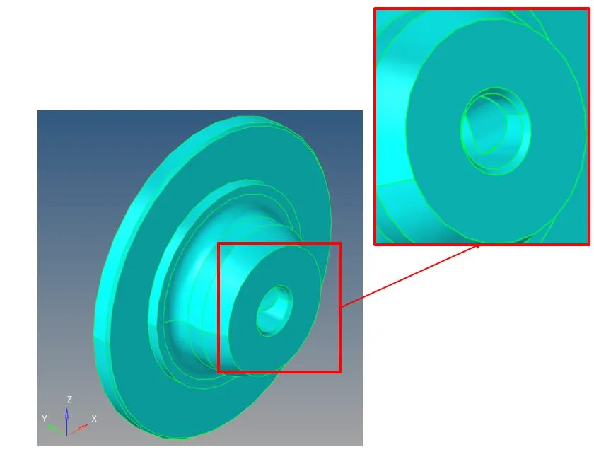
Fig 2.5: Hub

Since, the geometry is very complex, with lot of small features such as fillets and holes on the inside surface and thin gap between the hole and the fillet, using the hexa meshing is very difficult. If the hexa mesh is used, smaller elements has to be used, which decreases the time step size and thereby increases the simulation time. So the tetra mesh is used.

3D tetramesh can be performed by creating the 2D tria mesh and expanding it to 3D or can also create the 3D mesh of the component directly. For 3D tetra mesh,

3D → tetramesh

Fig 2.6: Volume tetra

In the “tetramesh” tool, volume tetra option is chosen. The surface of the component is selected and 2D element type of “trias” and 3D element type of “tetras” are chosen. Here linear tetramesh is used. So the element order is chosen as “first”. The element size of 5 mm is chosen.

Fig 2.7: Volume tetra

In order to maintain the element quality, in the “Tetramesh Parameters”, in the element quality section and “tet collapse” option, the value of 0.15 is chosen as the target value of the tet collapse.

Fig 2.8: Tetramesh parameters

Now the component is meshed.

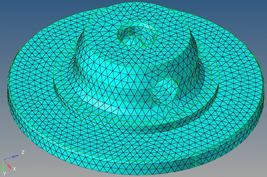
Fig 2.9: Tetramesh of Hub

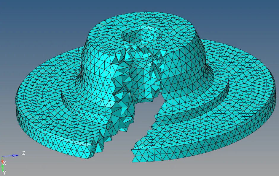
Fig 2.10: Tetramesh of Hub – cut section

From the cut section, it can be seen that the 3D mesh is successfully created with good transition among the features such as fillets and holes.

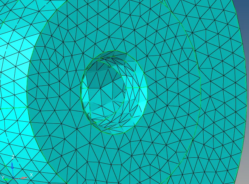
Fig 2.11: Tetramesh of Hub – fillets

The quality of the element created in hub is checked for any possible tet collapse. The element quality is checked here, to avoid wastage of time due to remeshing at the later stage. For checking the element quality “check elems” option from the “Tools” menu is used

Fig 2.12: Check elements option

Fig 2.13: tetcollapse

There were zero failed elements.

Now the second component cover is considered for meshing.

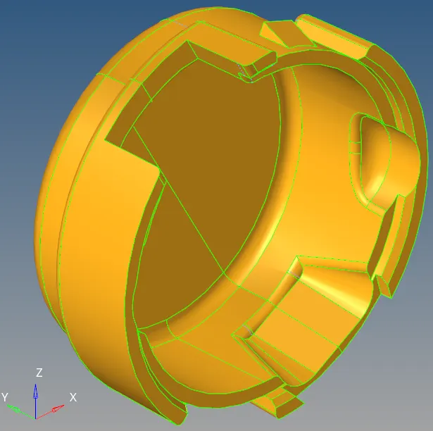
Fig 2.14: Cover

The same procedure as used for the hub is used to mesh the cover.

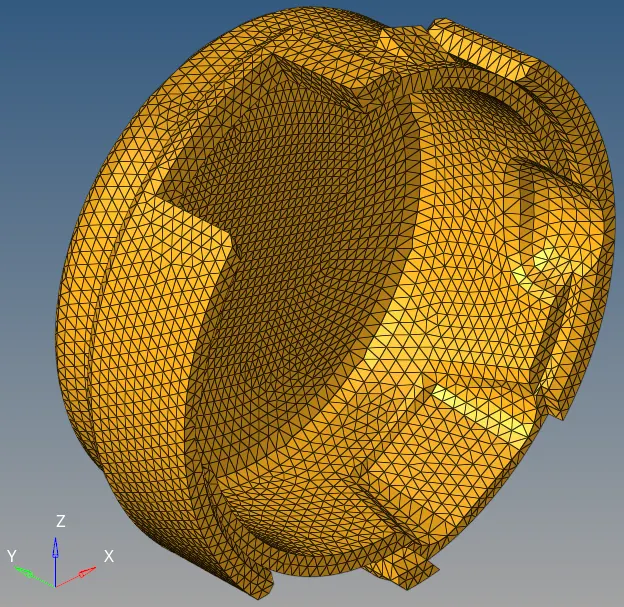
Fig 2.15: Cover – Tetramesh

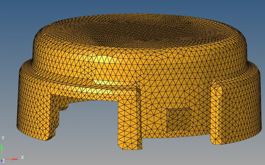
Fig 2.16: Cover – Tetramesh

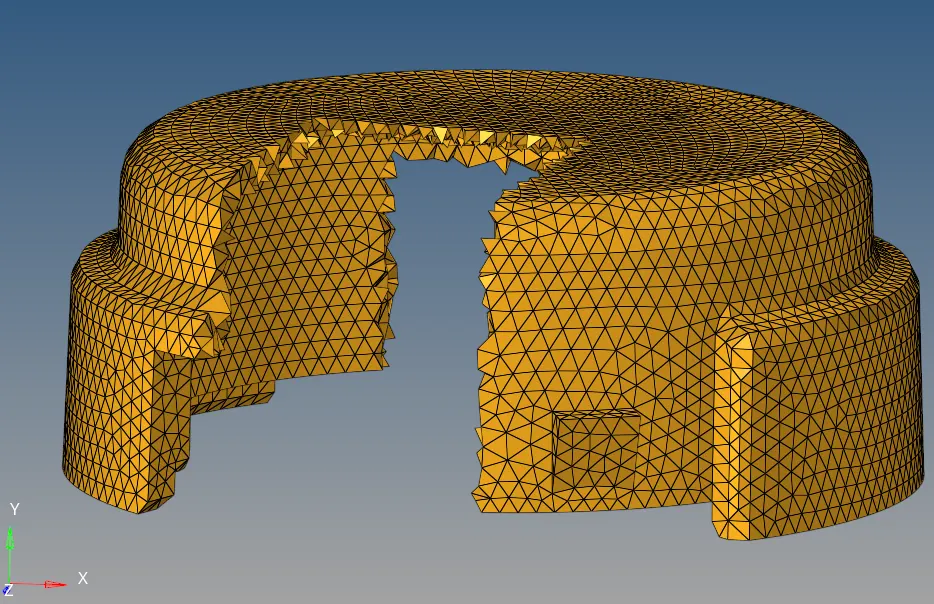
Fig 2.17: Cover – Tetramesh cut section

Fig 2.18: Cover – Tet collapse

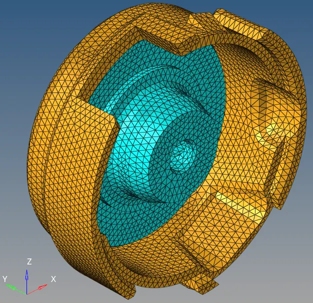
Fig 2.19: Final mesh of the entire assembly

The connectivity between the elements and the presence of any duplicate elements are checked.

Fig 2.20: Connectivity

Fig 2.21: Duplicate elements

Thus, the 3D mesh is performed for the assembly using the tetra elements within the required quality criteria of tet collapse being above 0.15 and the mesh is checked for any connectivity and duplicates.

3D Meshing - Arm Bracket:

The next component to be meshed is arm bracket.

Geometry:

The arm bracket consists of a rectangular base and a curved arm with the varying cross section and a hollow cylindrical boss at the top of it. Since it is solid component with the thickness greater than 6 mm and not a sheet metal component, solid elements are used for meshing.

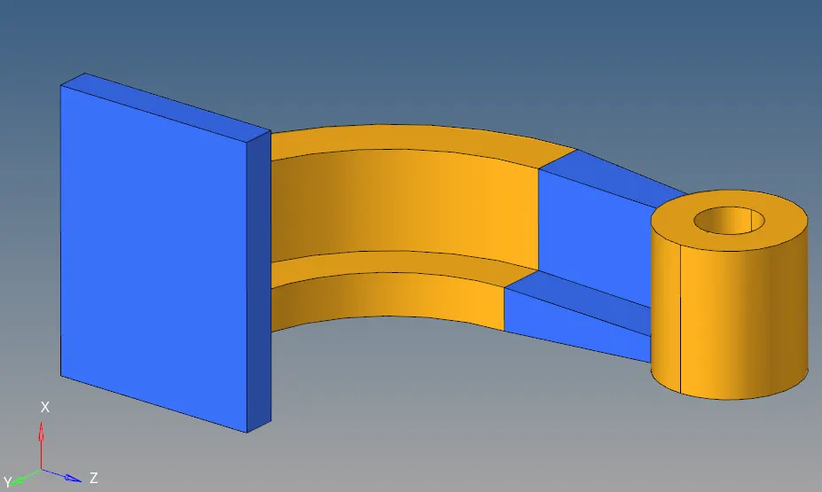
Fig 3.1: Arm bracket

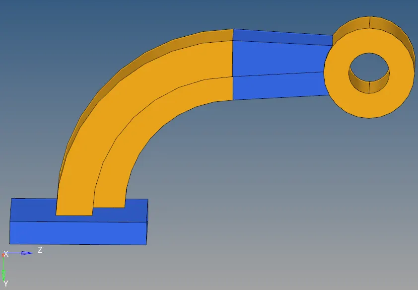
Fig 3.2: Arm bracket

Meshing:

Since it is solid component with the thickness greater than 6 mm and not a sheet metal component, solid elements are used for meshing. Since it is of varying cross section a 2D quad or tria elements has to be created and then it has to be extended along the edges of the various surfaces to get the final 3D solid mesh.

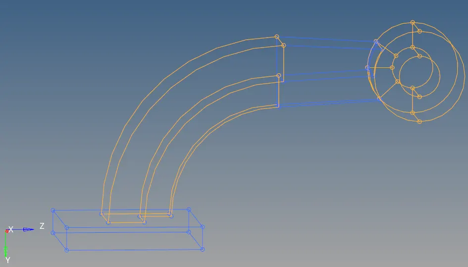
Fig 3.3: Arm bracket – wireframe representation

The arm bracket model has four components: base, arm curve, arm straight and a boss. Each has to be meshed separately. First the base is considered.

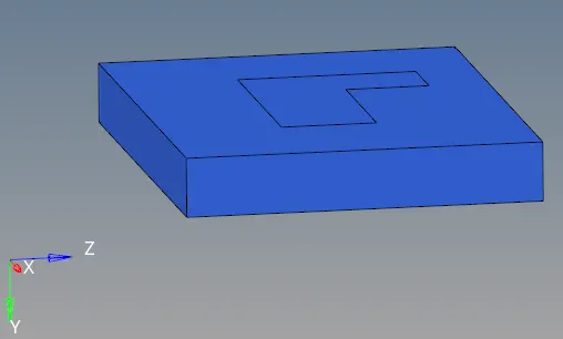
Fig 3.4: Base of the arm bracket

The 2D mesh is created on the base and then it is extended along the edge to create the 3D mesh. 2D quad elements are preferred to avoid the Penta6 elements, which are highly unstable. Penta6 elements are degenerated hex elements and will be mostly used in the transition regions such as transition from solid elements to the shell elements.

To create the 2D quad mesh on the base, “automesh” option from the “2D” tool is used. “quads only” is chosen as the element type to avoid any trais, which while extending create the Penta6 elements. The element size of 10 mm is used.

Fig 3.5: 2D automesh

Fig 3.6: 2D meshing parameters

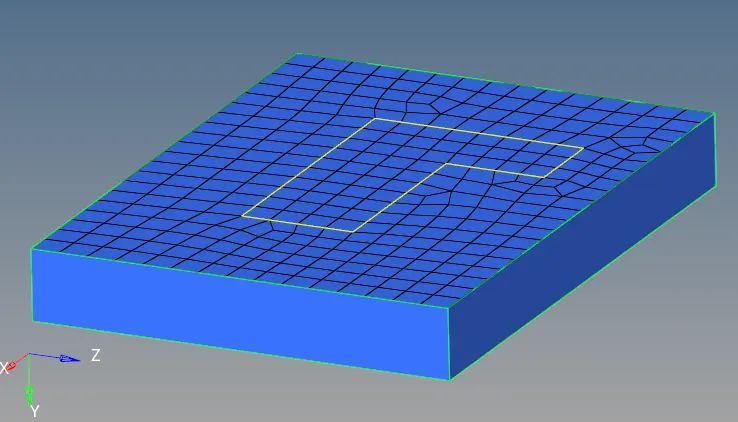
Fig 3.7: Base 2D meshed

Now this 2D mesh has to be extended to create the 3D mesh. For this “elem offset” option from the “3D” menu is used.

Fig 3.8: Element offset

The “solid layer” option is used. The elements on the top surface is selected and the surfaces along two perpendicular directions are selected for the “along geom to follow”. The thickness of the base is 25 mm and therefore number of layers along the surfaces are specified as 5, which will result in the hex element with the height of 5 mm.

Fig 3.9: Element offset parameters

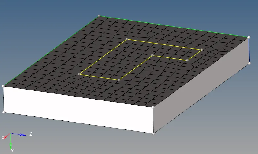
Fig 3.10: Mesh and along geom to follow selected

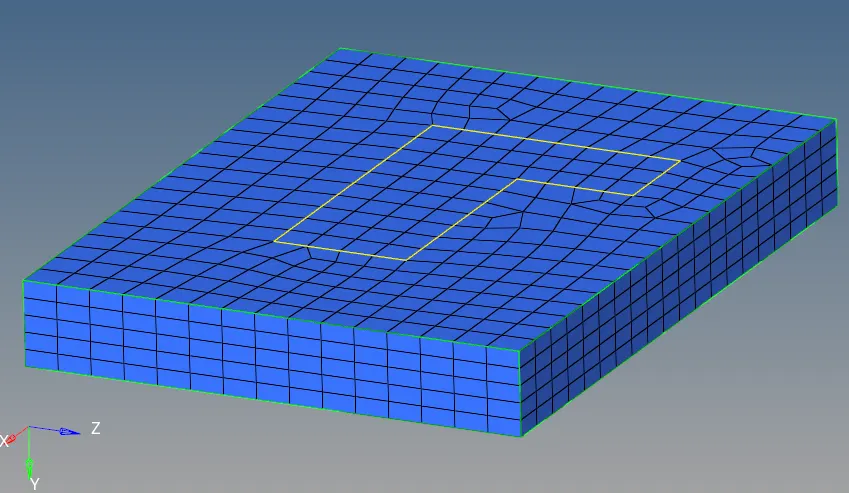
Fig 3.11: Base 3D mesh

Now the arm curve component has to be meshed. To mesh it, the 2D elements created at the center surface of the base will be used.

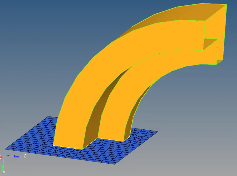
Fig 3.12: Arm curve with 2D element from the base

Since the surface is curved “spin” option from the “3D” menu is used.

Fig 3.13: Spin option

Fig 3.14: Spin option parameters

The elements at the center surface, which is at the shape of cross section of the arm curve, are selected. For the axis of rotation, the center of the circle of any curved surface and x-axis is chosen, along which the component is perpendicular. Angle of 90 deg and 25 elements along the spin are chosen.

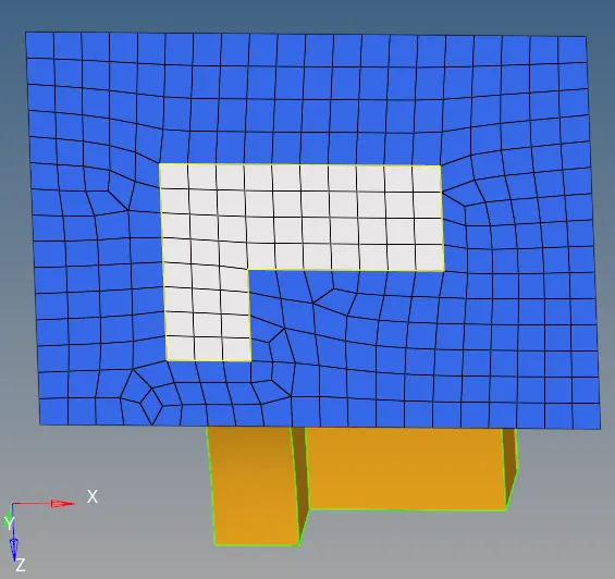
Fig 3.15: Elements selected for spin

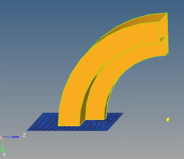
Fig 3.16: Centre of the curve

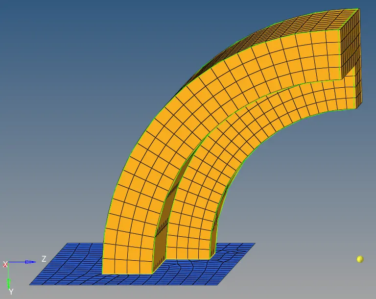
Fig 3.17: Final mesh

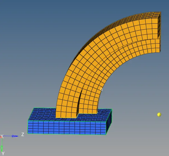
Fig 3.18: Base and arm curve meshed

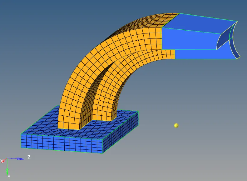
Fig 3.19: Base and arm curve meshed with arm straight

For meshing the arm straight “linear solid” option from the “3D” tool is used. For this, 2D mesh is needed at the end of the arm curve. For that 2D, the faces of the mesh on the arm curve is needed. It is extracted using the “Faces” option from the “Tools” menu.

Fig 3.20: Faces

Fig 3.21: Faces parameters

For components, arm curve is chosen.

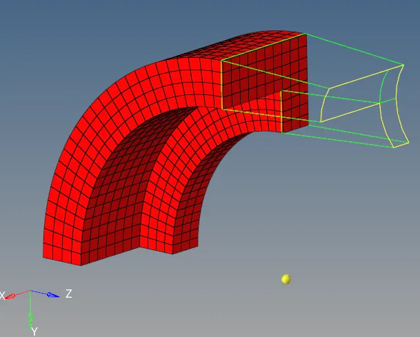
Fig 3.22: Arm straight with the faces of the arm curve

Now the “linear solid” element option from “3D” is used for meshing the arm straight, since it is tapered in nature.

Fig 3.23: Linear solid option

Fig 3.24: Linear solid option

For meshing using the “linear solid” option, elements are required at the destination face. So firat 2D mesh is created at the end face of the arm straight component using the “automesh” option from the “2D” tool using the “quad only” option and the element size of 10 mm.

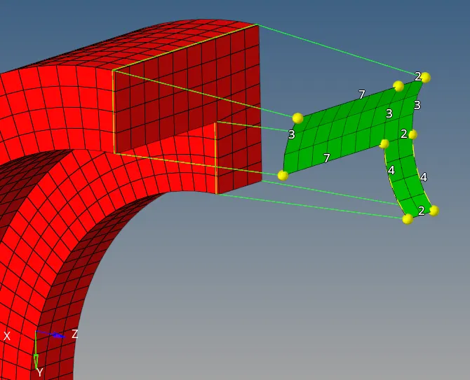
Fig 3.25: Initial 2D at the end face of the arm straight

The number of elements at the start of the arm straight i.e. end of arm curve and the end of arm straight has to be same to avoid the Pents6 elements.

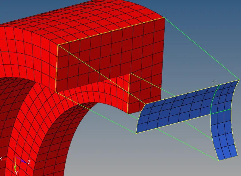
Fig 3.26: Final 2D at the end face of the arm straight

Now the “linear solid” option is used to extend the mesh from the end of arm curve to end of arm straight.

Fig 3.27: linear solid parameters

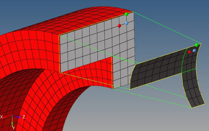
Fig 3.28: linear solid selection

For “from” elements at the end of the arm curve and for “to”, the 2D elements at the end of the arm straight are selected. For the alignment 3 nodes on the face of arm curve elements are chosen and the same corresponding nodes are chosen on the 2D elements at the end surface of arm straight, to signify that the nodes will be transported from there to the new position.

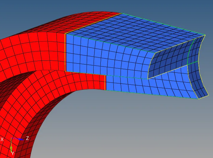
Fig 3.29: Arm straight mesh

Now the face created is deleted.

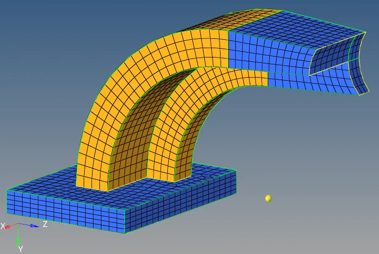
Fig 3.30: Base, arm curve and arm straight meshed

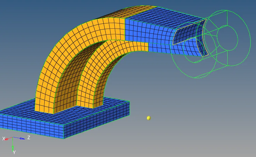
Fig 3.31: Base, arm curve and arm straight meshed with boss

For boss, the “solid map” option from the “3D” menu is used. For this the source mesh is required. Thus, 2D mesh is created at the one circular face of the boss using “automesh” option from “2D” menu.

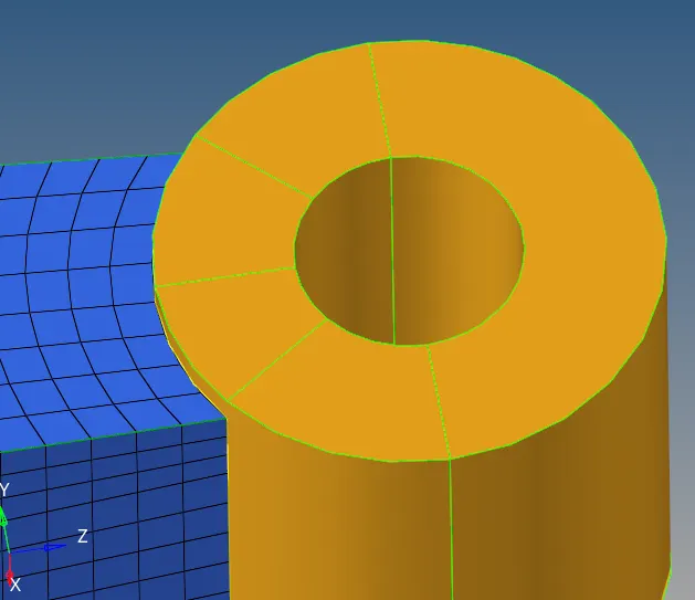
Fig 3.32: Boss surface before 2D mesh

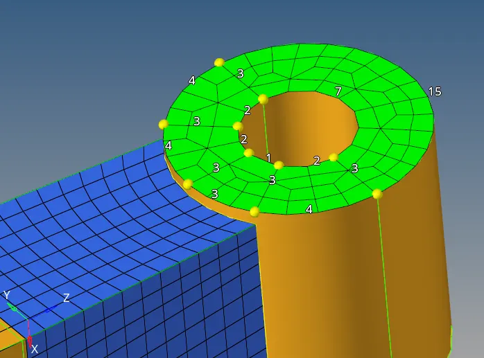
Fig 3.33: Boss surface after automesh

The mesh created are not uniform. In order to improve the mesh flow, number of nodes on the upper and the bottom sides are made equal.

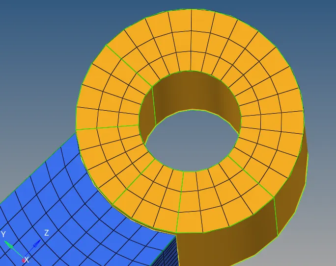
Fig 3.34: Boss surface final 2D mesh

For using solid map option, nodes are required along the path till the end surface to guide the elements. Thus a node created at the other circular surface of the boss using “project” option from “tools” menu.

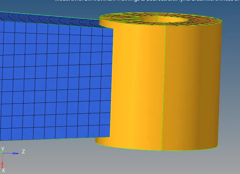
Fig 3.35: Before the node generation

Fig 3.36: Project option

Fig 3.37: Project option selection

Node belonging to the end mesh of the arm straight and the required circular surface is selected. “along vector” is chosen as “surface normal” to create the node at exactly the same location as of the end node on the destination surface.

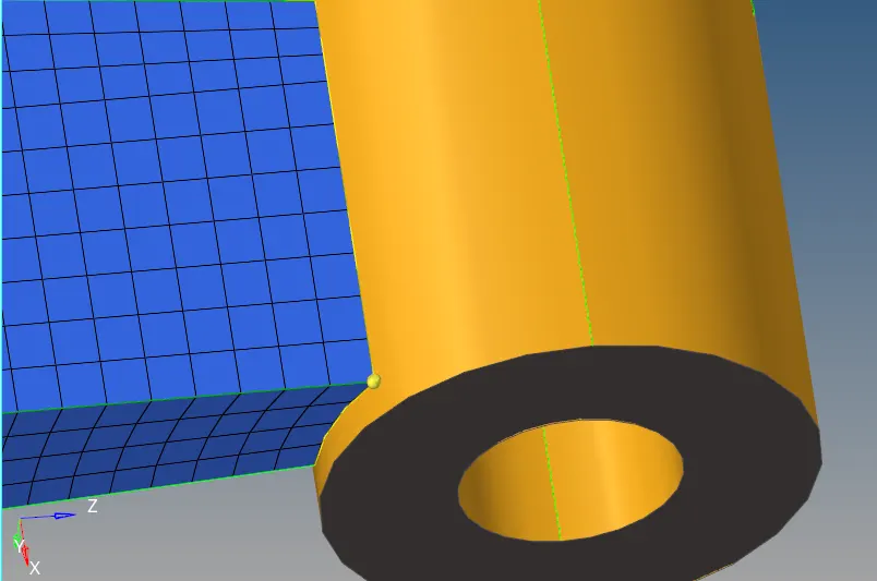
Fig 3.38: Project option selection

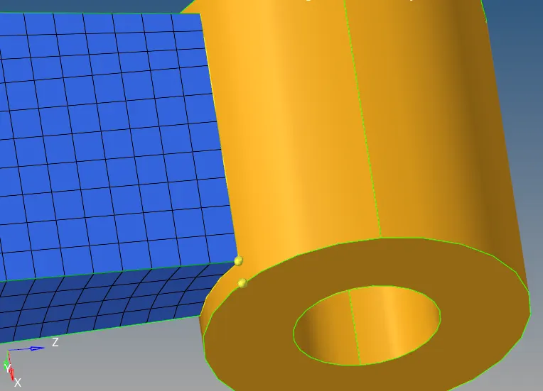
Fig 3.39: After node generation

Using this “solid map” option can be performed to create the 3D mesh along the cylindrical face of the boss.

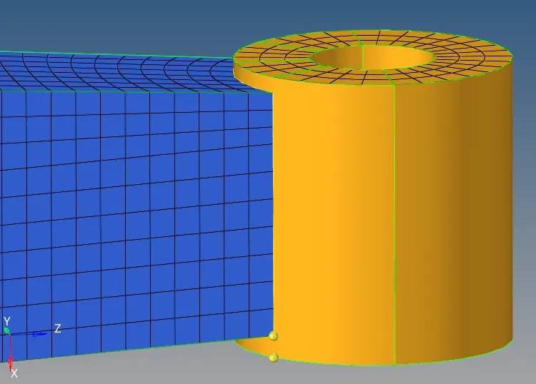
Fig 3.40: Before solid map

Fig 3.41: Solid map option

Fig 3.42: Solid map selection

The 2D elements created on one of the circular face is selected for the “elem to drag” and the circular face at the other end is selected as the “dest geom”. The node on the 2D mesh and nodes of the elements at the end of arm straight and the node created through “project” selected for “along geom”, which will guide the source elements to the destination surface and it will also ensure connectivity with the elements on the arm straight.

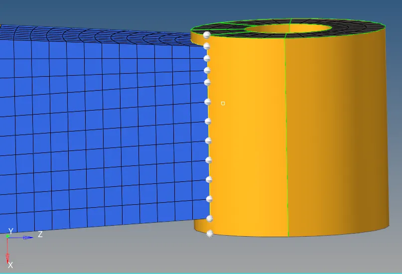
Fig 3.43: Node path for solid map

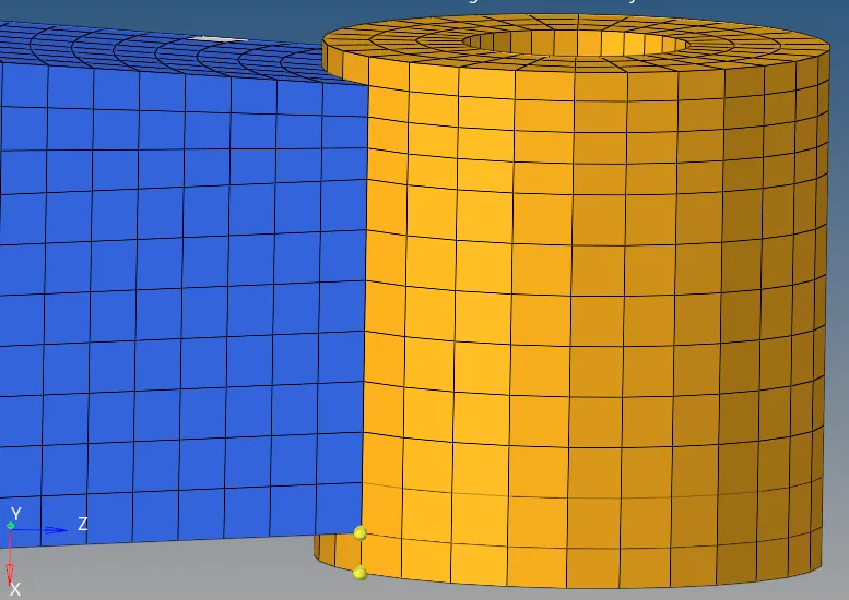
Fig 3.44: Boss meshed

From the fig 3.43, it can be seen that the elements are created along the cylindrical face of the boss with the good mesh flow and also ensuring the connectivity with the elements of arm straight. The 2D elements created are deleted to avoid the duplication and calculation errors during the simulation.

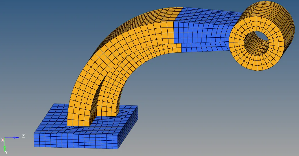
Fig 3.45: Final meshed component

The final mesh is selected for any connectivity or any possible duplicates using “check elems” option from “Tools” menu.

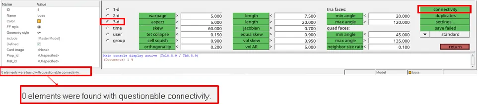
Fig 3.46: Connectivity

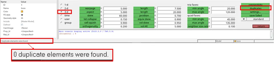
Fig 3.47: Duplicates

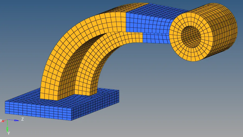
Fig 3.48: Meshed component

Thus, the 3D mesh is performed for the assembly within the required element quality criteria. Here the meshing is performed such that the Penta6 elements are avoided. Therefore the component is meshed thoroughly using the hexahedron elements, thereby achieving the good mesh quality.

Conclusion:

The basics of the starter input deck (FIRST_RUN_0000.rad) and the engine input file (FIRST_RUN_0001.rad) has been explained in detail. The speed of the sound in steel and the time taken by the sound wave to travel through the length of the steel rail has been successfully calculated. These calculated values are given as the termination time and the frequency of the animation output in the engine input file by editing the .rad file directly and by using the Radioss solver deck browser. The resultant listing files (.out files) of both the starter input deck and the engine input file has been obtained and given in the report.

Then the two components (housing and the arm bracket) are meshed using the 3D solid elements (tetrahedron and hexahedron) with in the required quality and mesh flow. The mesh is performed such that the tet collapse value lies above 0.150 and to avoid the Penta6 elements, because they are highly unstable element.