Challenge

Assignment 3-2D Element Formulation Challenge

Solution of question 1:-

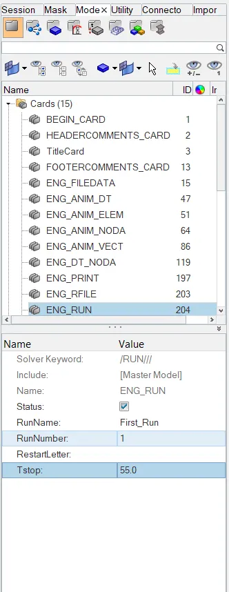
to change the run time first imported the solver deck into HyperMesh (0.rad file/ starter file)
then I clicked on the "cards" of the model in the model browser
then I selected the Eng_Run property
then a drop-down appeared where I changed the "Tstop" from 60 to 50ms as mentioned in the question

Browser--> Model--> Cards--> Eng_Run--> Tstop

Solution of question 2:-

to change the number of animation steps during simulation to a minimum of 25 and a maximum of 60.
I selected the value of in between which is 55
so as we know to change the number of animation steps during simulation we need to calculate the Tfreq and we have the change the Tfreq value to change the number of animation steps during simulation.
So as we know the formula

Δt= l/c ......equation 1
and Tfreq= Δt/number of animation steps ......equation 2
So,
Δt = 55 ms given in the question
by using equation 2 I calculated the Tfreq value which is
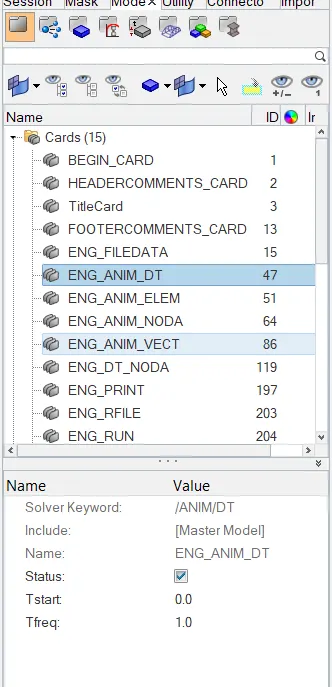
Tfreq= 55/55
Tfreq= 1
So to change the Tfreq value
followed the same procedure as above but this time instead of the ENG_Run card I used the ENG_ANIM_DT
And there changed the Tfreq to "1".

Solution of question 3:-

To run the base simulation
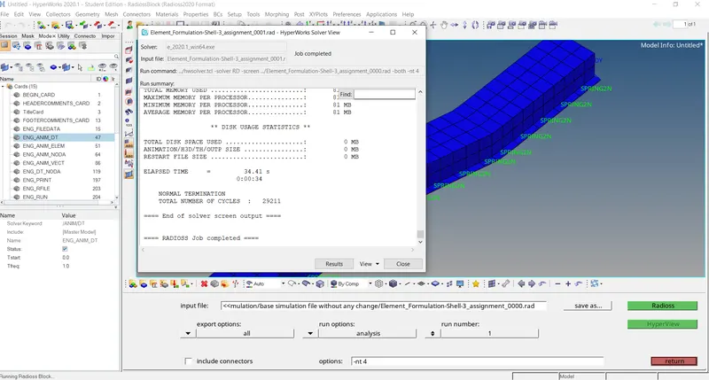
opened the RADIOSS from Analysis
then in options wrote "-nt 4" where nt means no. of threads and the complete meaning of this is that it is using 4 CPUs together to solve the file
Then clicked on RADIOSS
It saved all the simulation files in a local directory of our computer

Solution of question 4:-

To check the Energy or mass error
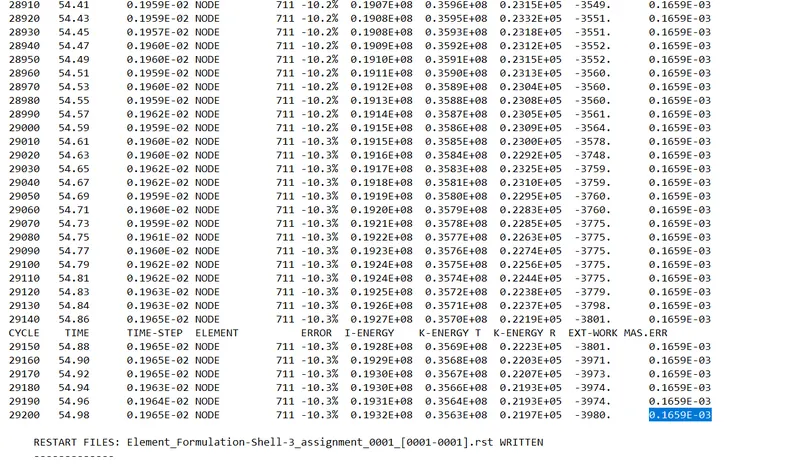
opened the 1.out file which was created after running the base simulation
The energy error is between 0% to -10%
which is under the acceptable values
and the mass error is also 0.1659E-03 throughout the simulation which is acceptable

Solution of question 5:-

So as the energy error and mass error are acceptable so we can plot rigid wall forces, hourglass energy, internal energy, contact energy, and total energy using HyperGraph 2d
So first I opened the HyperView to run the simulation and observe the component while the deformation
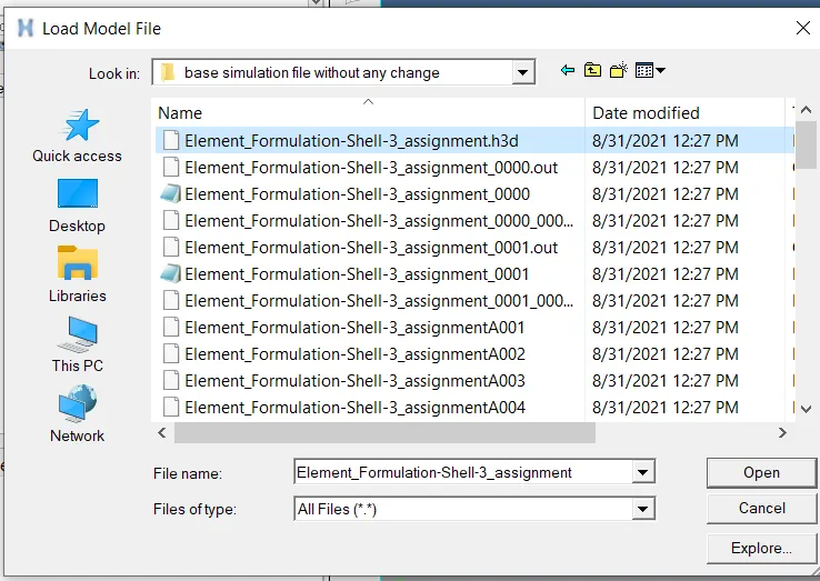
After opening the "h3d" file in HyperView
there we can easily see the deformation by just clicking on the run button
So after observing the deformation one can conclude that hourglass is happening in few areas.
So now to Plot the rigid wall forces
I opened the HyperGraph 2d then
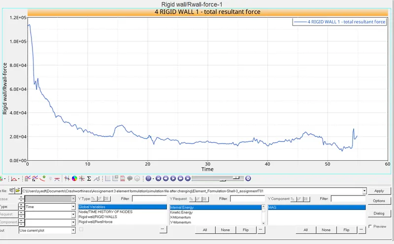
There I opened the T01 file to plot the rigid wall forces

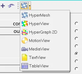
HyperView from where I opened the H3d file
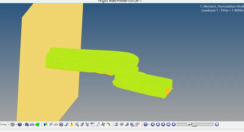
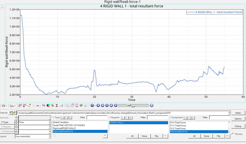
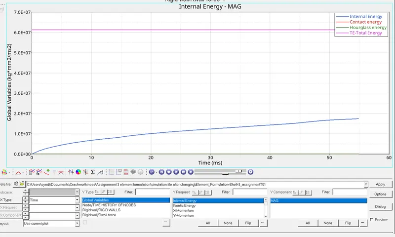
Similarly to plot the Energy graphs I opened the global variables instead of rigid wall forces and then selected all the three energies

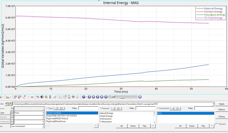
OUTCOMES 1:-
Few Conclusions that can be made out of these graphs are:-
- Internal Energy is gradually increasing it may be because of the force developed due to deformation
- Then total energy is decreasing slowly
- Hourglass energy is increasing its because as observed in the simulation too, some elements are deformaing in very unrealistic manner and the element size is also large and because of the type of element used in this simulation has very less number of Gaussian Integration Points
- And Contact energy was almost constant throughout the simulation

Solution of question 6:-

to change all the shell element properties first I openened the Starter (0.rad) file into HyperMesh
then there in the Property cards changed the values of Ishell, Ismstr, Ish3n, N, Ithick, and Iplas.
then after changing the values followed the same procedure as above
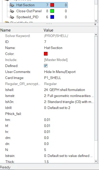
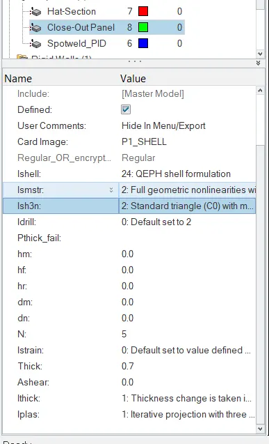
Then after this by using the RADIOSS tool from analysis saved the file into another new folder
then I checked for energy and mass error by opening the 1.out file
there I found that the change in shell element properties has really decaresed the energy and mass error which is a very good sign
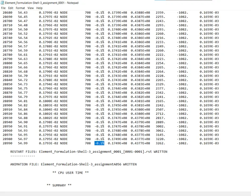
In this the energy error was in between 0% to 0.1% which is very good and mass erros was 0.1659E-03 which is also acceptable and less than previous one
Then after analysing energy and mass error
I plotted Rigid wall forces and the global variables using the T01 file created after saving the RADIOSS file
So to plot the graphs I followed the same procedure as for the above

OUTCOMES 2:-

So from these plots the conclusions that can be made are
- because of using QEPH elements this time there is no hourglass energy because the QEPH element has more number of Gausssian Integration Points which eliminate almost all the possibilities of having any hour glass energy
- And then the Rigid wall force graph force is also more accurate as we can see initially the force is at peak because the deformation hasn't started yet but within a very few seconds the force decreases and then starts to change very slowly this is because of the stiffness of the component and then when the deformation reaches at the angle it decareses
- The total energy is constant throughout the smilution which indicates no energy error
- Then the contact energy remains 0 throughout the simulation

Conclusions:-

Ship work like this
in your own course.