Assignment 3-2D Element Formulation Challenge
Aim:
1) Start the experiment with Case 1, the default property card.
2) Modifying the Case 2 property card
3) Comparing the prerequisites for Cases 1 and 2
Component Deformation,
1D: Contains beams, springs, and trusses.
2D: Contains shell components such as TRIAS and QUADS.
3D: Contains solid components like TETRA and HEXA elements.
Key parameters
Ishell:-To choose the element formulation for shell elements with four nodes.
Ish3n:-To choose the element formulation for shell elements with three nodes.
N: Selecting how many integration points to pass through the thickness
Ismstr: To indicate if the formulation of strain is modest or large.
Iplas: To determine the post-yield strain calculation technique.
Ithick: To ascertain if the element thins or whether the thickness remains constant under stress.
Case 1:- WITHOUT DESIGNATING THE PROPERTY'S RECOMMENDED PARAMETER
1) Open the RADIOSS user interface and import the model.
2) Open the file in SOLVER DECK format.
3) The model will resemble this
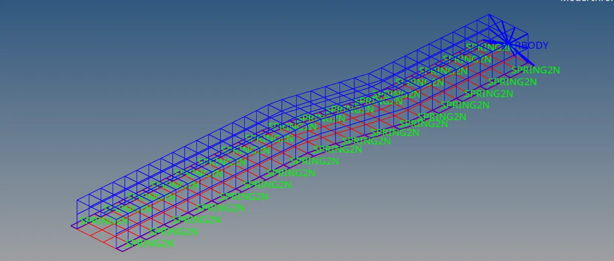
4) The next action is to set the time step value in ENG_RUN vehicles to 55 ms in accordance with the query.
5) The number of animation steps has now been assigned. In response to the query, I decided on 50 ms as the animation step length.
Frequency= NUMBER OF ANIMATION STEPS / TIME STEP = 55/55 = 1.
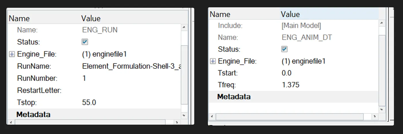
6) Each parameter property is displayed below by default in the property card.
7) The simulation ANALYSIS—RADIOSS will now be executed.
8) It is advised to use -nt 4 in the RUN OPTION panel. This does not indicate the number of threads that are assigned to completing the simulation more quickly.
9) When you click Radius, the message "Job Completed" appears.
10) Click RESULT at this point to be sent straight to Hyperview, where we can witness the simulation's animation. The animation files are named h3d & Click apply
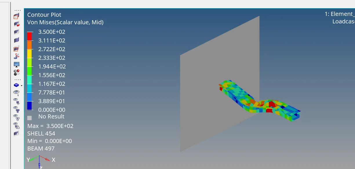
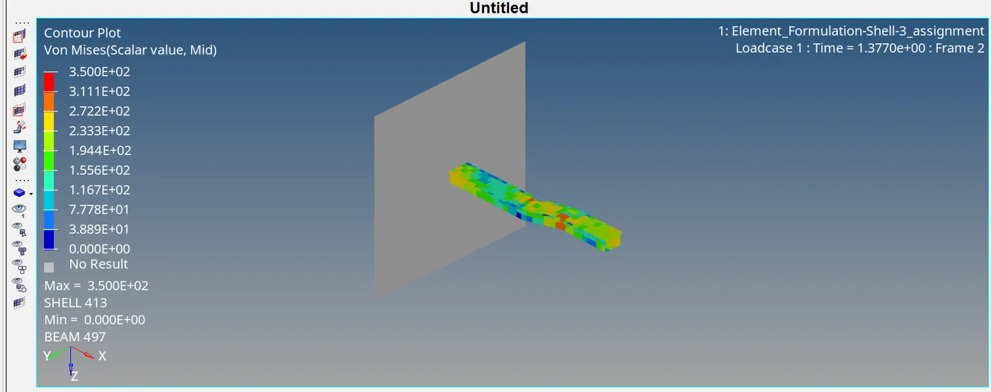
11) To view the deformation, choose the RESULT TYPE after switching. I choose VON MISSES and hit submit.
12) Plotted graphs for the different energies. To plot a graph, select the Hypergraph tab and import the T01 file, which represents the time history.
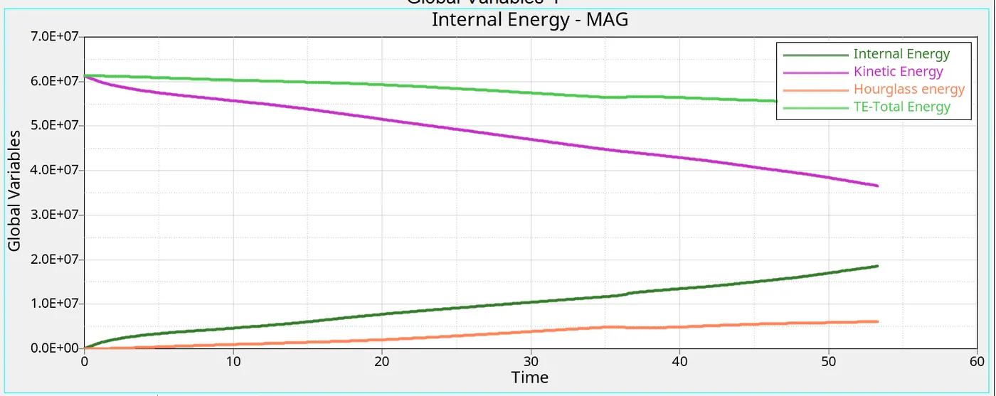
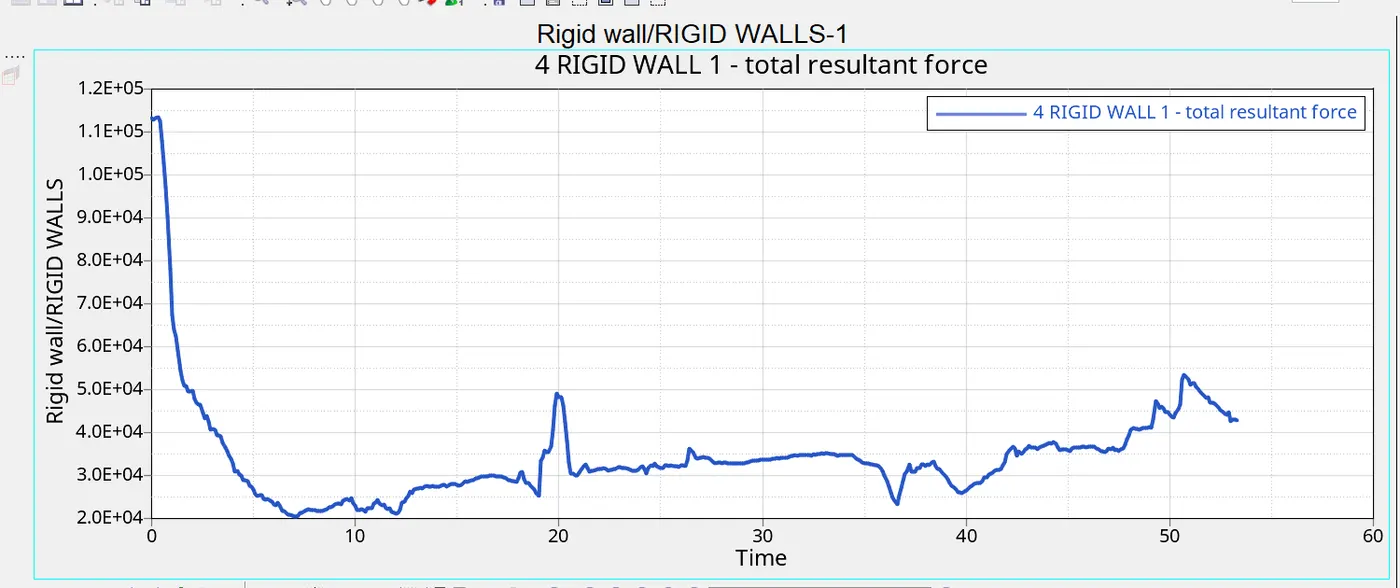
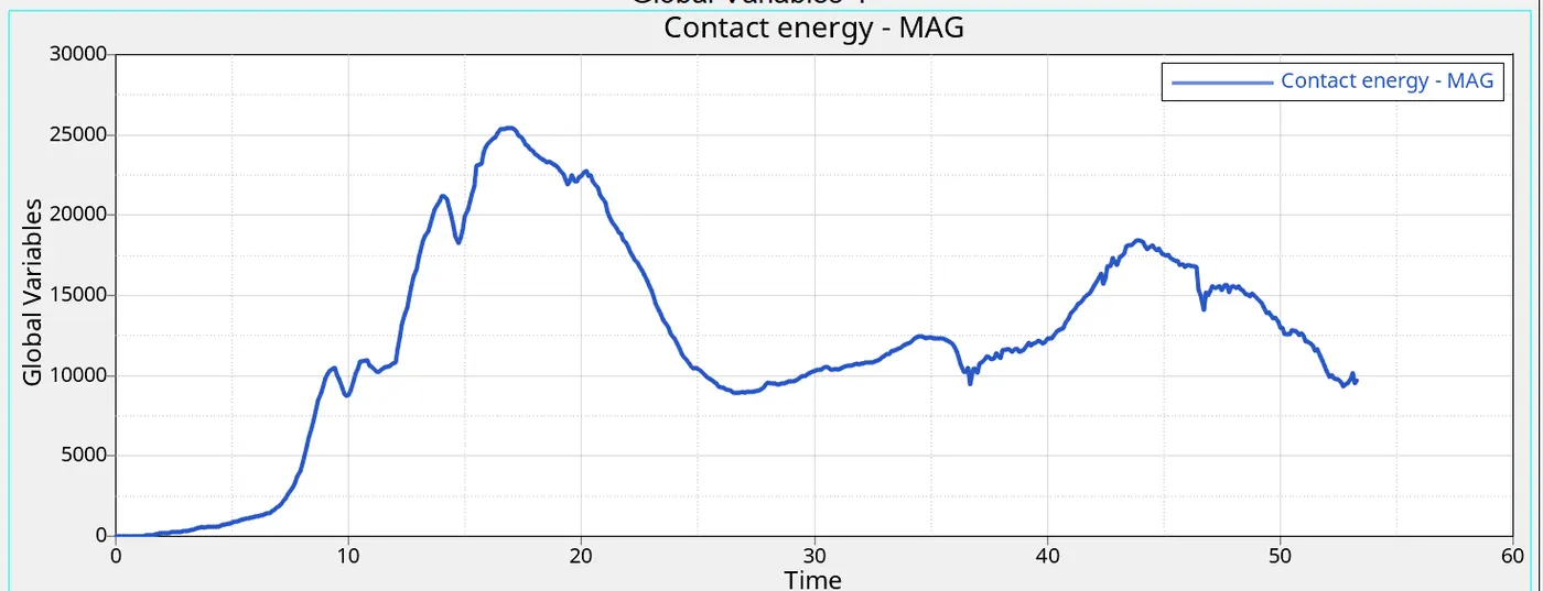
The following observations are drawn from the plot produced by the base simulation in which element characteristics were left unchanged:
Because of the force that deformation places on the tube, internal energy accumulates during the simulation.
Over the course of the simulation, hourglass energy slightly increases.No contact energy is created throughout the simulation.
From the beginning of the simulation to the finish, the system's total energy slightly decreases.
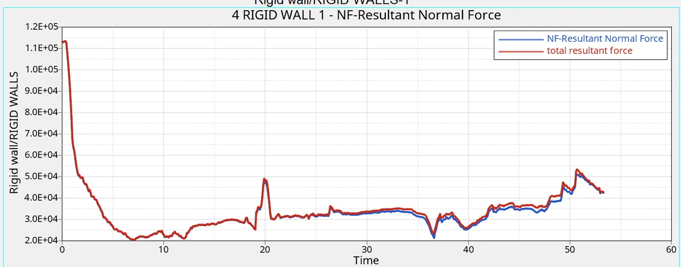
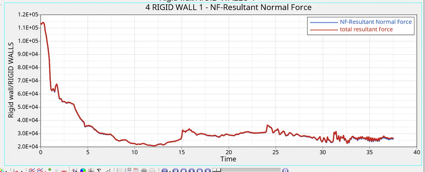
A new plot is created to plot the rigid wall forces.
The above plot of total resultant force and resultant normal stiff wall forces against time illustrates this.
Because of the fluctuating force that the crush tube applied to the wall during the simulation, the stiff wall force curve exhibits nonlinear behavior.
Case 2: Changing the shell elements properties to recommended properties
Ishell =24 QEPH 4 nodes shells are the best combination of cost and accuracy.
Ismstr = 2 Full geometric nonlinearities (default)with possible small strain formulation activation in RADIOSS Engine.
Ish3n = 2 Standard 3 noded shell (C0)with modification for large rotation(default)
N=5 Number of integration points set to 5 for accuracy bending.Thick=1
Thickness change is taken into account for accuracy.
Iplas = 1 Iterative plasticity for good accuracy
The attributes of the shell elements are changed to the following suggested values:
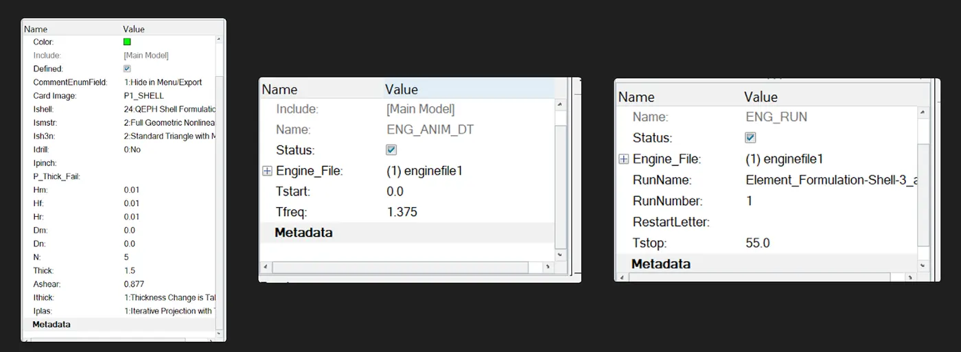
1)Adding 55 ms to the run time
2) The Tstop for the ENG_RUN card has been adjusted from 60 to 55 in the model tree under the CARDS collector.
3) Adjusting the animation steps to forty:
4) The frequency for 40 animation steps is run time/animation steps = 55/40 = 1.375.
5) The Tfreq for the ENG_ANIM_DT card has been adjusted from 1.0 to 1.375 in the model tree under the CARDS collector.
6) Using the Radioss option under the Analysis tab, run the simulation using the newly established suggested settings. In the edit options, set the thread count to "-nt 4 ".
7) The.OUT file is examined following analysis to see if the mass and energy errors are within an acceptable range.
8) Plotted graphs for these different energies. To plot a graph, select the Hypergraph tab and import the T01 file, which represents the time history.
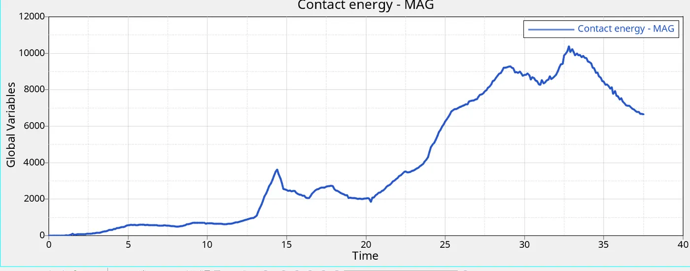
9) The energy inaccuracy is within an acceptable range, ranging from 0% to -0.10%.
10) The mass error remains within the permitted range, at 0.1659e-03, throughout the run.
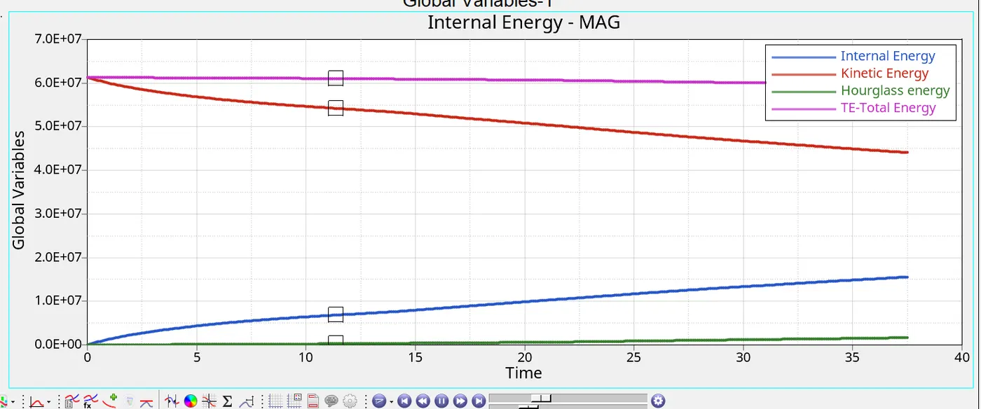
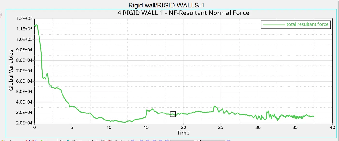
11) The stiff wall forces, internal energy, hourglass energy, contact energy, and total energy of the simulation are shown using hypergraph 2-D since the error levels are acceptable.
12) Open the file Element_Formulation-Shell-3_assignmentT01. On the same figure, as indicated below, specific energies are plotted versus time,
13. Throughout the simulation, internal energy rises as a result of the force that deformation places on the tube.
14) Throughout the simulation, the total energy stays constant.
Throughout the simulation, hourglass energy and contact energy are always zero and follow the origin.
Comparison:-
The energy error, which was -10% but has since corrected to -0.1%, indicates that total energy is still constant rather than declining.
Throughout the experiment, the growing hourglass energy changed to zero.
The properties of contact energy are the same in both situations.
In both situations, internal energy is gradually gaining characteristics.
Additionally, rigid wall forces dropped to a number that was less than the rigid wall force value set by default.
Contour plots demonstrate that the maximum displacement of an element with suggested property values has somewhat increased.
Hourglass energy
Since the deformation energy of components in the hourglassing mode is zero, the hourglass mode is sometimes referred to as the "zero energy mode" in FEA. However, the energy of the hourglass is not zero.
A reduced integration that employs a single integration point is utilized in a shell element with many integration points to decrease computing work. The deformation mode derived from the analysis findings will be erroneous in these situations. It's known as the hourglass phenomenon.
All that's happening here is a non-physical zero energy phase that causes extreme element distortions. The better the outcome, the more organized and less distorted your elements are.
In order to address this issue,
a) One remedy is mesh refining. In coarse mesh, hourglassing is more common.
b) Although fully integrated components are prone to shear locking and require significantly more computing time, they are still preferable.
c) Supplying a little, arbitrary stiffness in the hourglass deformation phase. There is no such rigidity in the real physical system; this is only a FEA point of view. The term "built-in hourglass controls" refers to this.