Assignment 3-2D Element Formulation Challenge
AIM: The main aim of this challenge is to run the crash beam base simulation without modifying the element properties and compare this simulation results with the base simulation by changing its properties.
OBJECTIVE: The objectives of this challenge are as follows:
1. To change the run and frequency time as per the given question and run the base simulation without changing any elemental properties.
2. To run the base simulation as per the recommended properties given in the question.
3.To post process all the results and compare both the cases.
PROCEDURE:
CASE-1: No change in elemental properties
1. The _0000.rad file can be imported by using import solver deck option.
2. The run time (SOLVER BROWSERàENGINE_KEYWORDSàRUNàTstop =55) for the simulation should be updated to 55ms. Run time can be edited by using hyperworks or can be directly edited from _0001.rad text file. If we are directly editing from the text file, we need to be more cautious about number format.
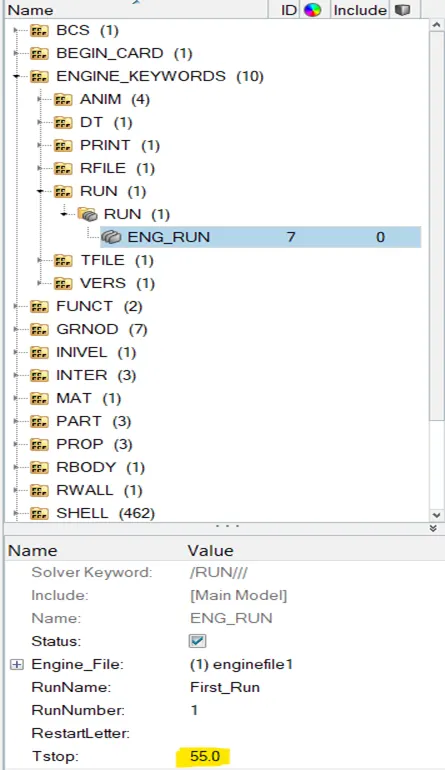
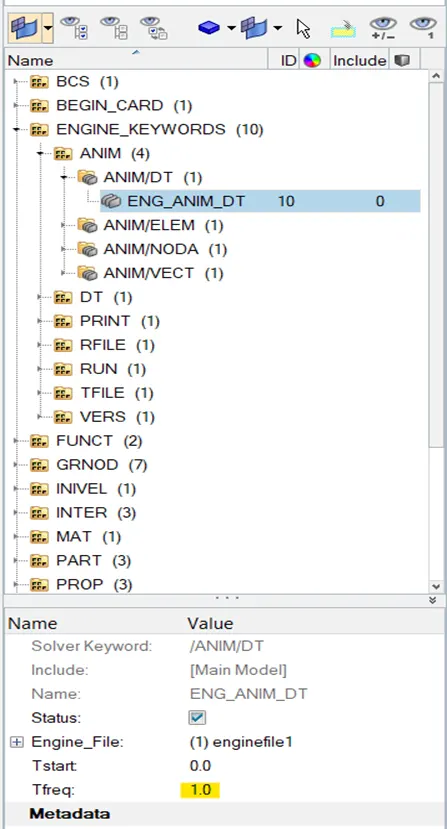
3. 55 animation steps were considered, and for 55 animation steps frequency time calculation is shown below.
Tfrequency= Run time/animations required=55/55=1ms.
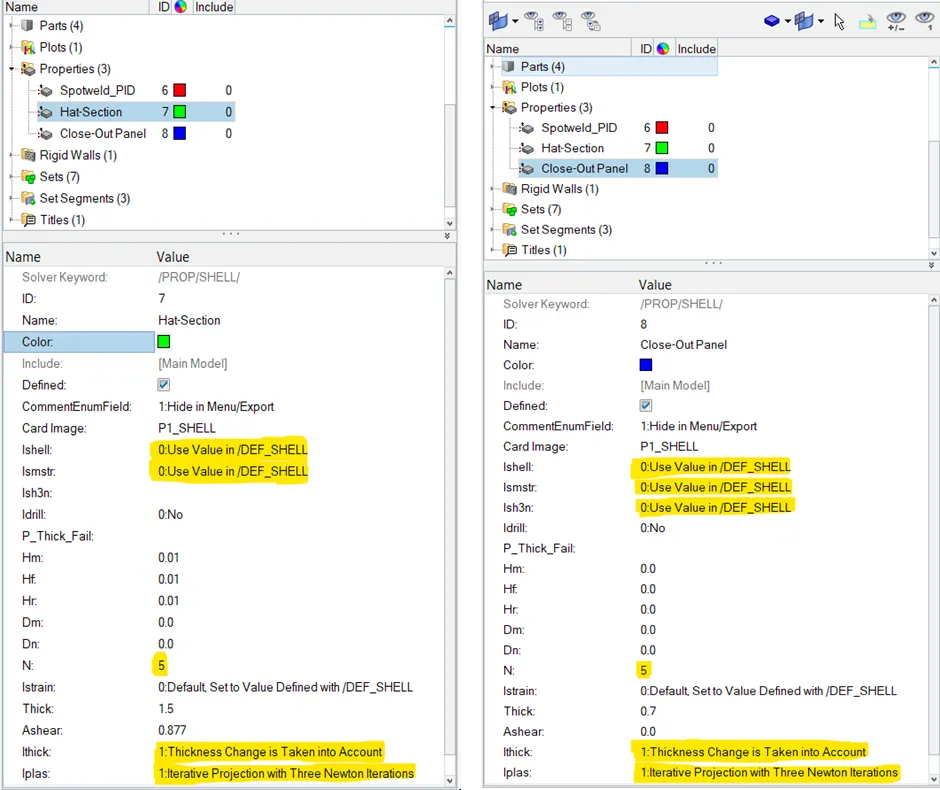
4. Initial default properties of 2D elements are shown in the below image.
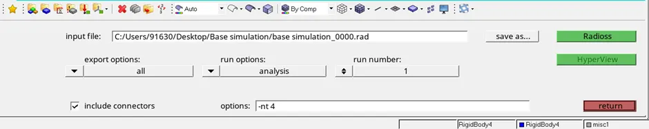
5. Save the file and run the analysis. (ANALYSISàRADIOSS).
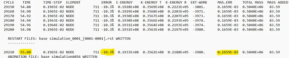
6. Check for mass and energy errors in _0001.out file. Energy error can range from -15% to +5%. The energy error at the end of the simulation was found to be -10.3% and mass error was very negligible.
7. Simulations and graphs will be shown in the comparison section.
CASE-2: Changing the elemental properties as per recommended properties.
1. The _0000.rad file can be imported by using import solver deck option.
2. The run time (SOLVER BROWSERàENGINE_KEYWORDSàRUNàTstop =55) for the simulation should be updated to 55ms. Run time can be edited by using hyperworks or can be directly edited from _0001.rad text file. If we are directly editing from the text file, we need to be more cautious about number format.
3. 55 animation steps were considered, and for 55 animation steps frequency time calculation is shown below.
Tfrequency= Run time/animations required=55/55=1ms.
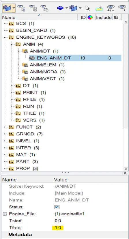
4. Recommended properties of 2D elements are shown in the below image.
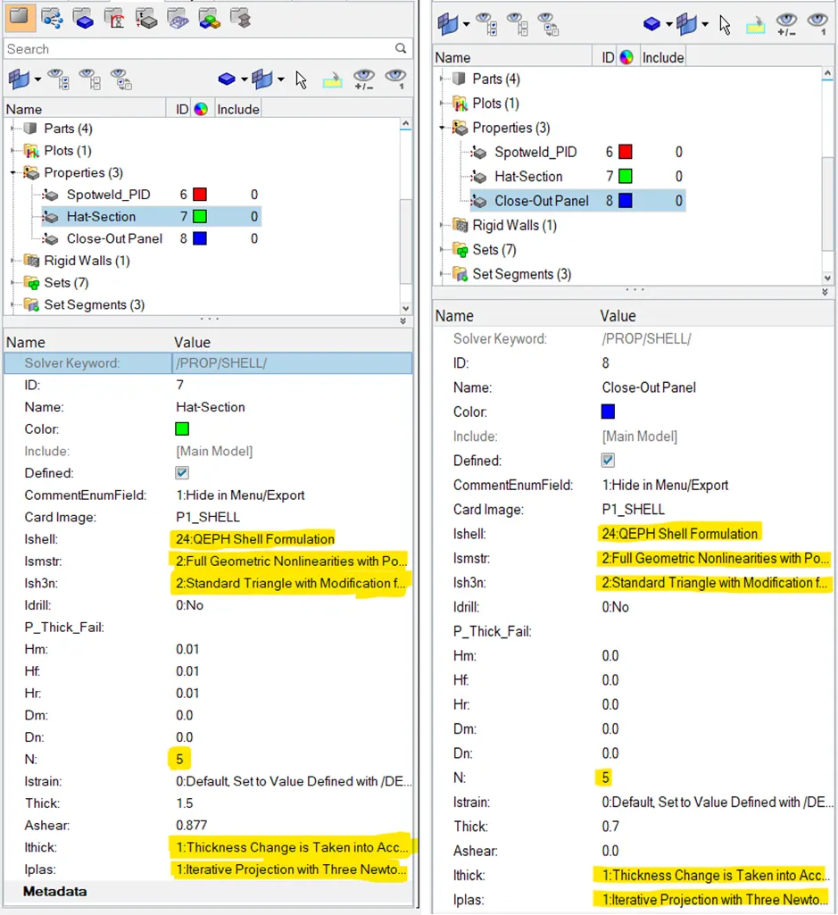
5. Save the file and run the analysis. (ANALYSISàRADIOSS).

6. Check for mass and energy errors in _0001.out file. Energy error can range from -15% to +5%. The energy error at the end of the simulation was found to be -0.1% and mass error was very negligible.

7. Simulations and graphs will be shown in the comparison section.
RESULTS COMPARISION:
Variation of Energies and Forces:
Case-1
Case-2
Case-2
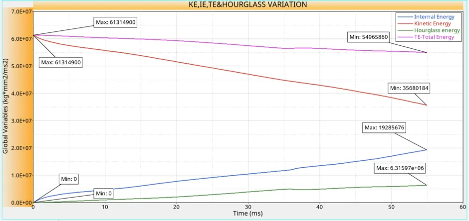
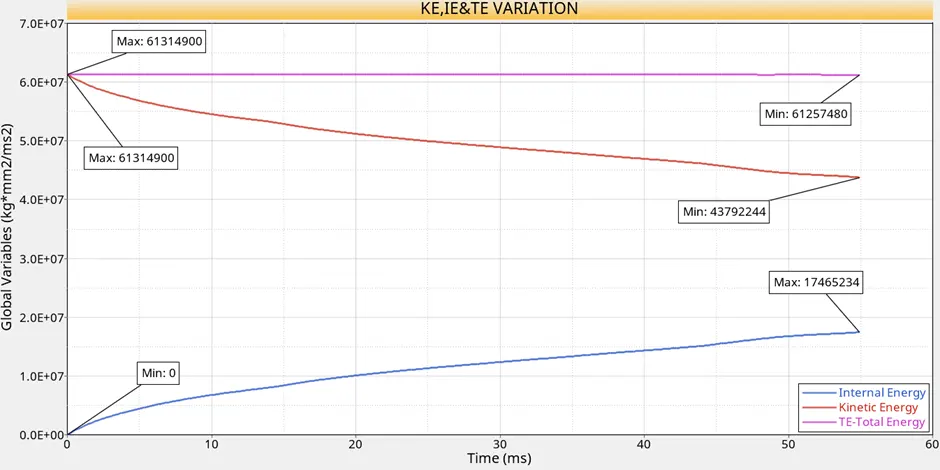
Kinetic Energy: Since the component was moving with some initial velocity, the component was having some KE at the starting of the simulation and the same thing was depicted in both the cases graphs. As the simulation time increases the deformation in the component will start and this KE will be converted internal energy to maintain energy balance. This was correctly depicted in the graph for both the cases. Because of the more realistic deformation in second case min value of K.E at the end of the simulation was high compared to case-1.
Internal Energy: The amount of work done to deform any body will be stored as energy inside the body and this energy is called internal energy. If the deformations are more then the body will have more internal energy. Initially there was no deformations in the rail component, therefore the internal energy in both the cases started from zero. As the simulation time increases, the deformation in the rail component also increases leading to increase in internal energy variation of both the cases.
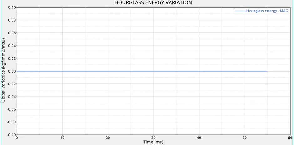
Hourglass Energy: It is an artificial form of energy that occurs in first order elements having reduced integration points. It is a zero-strain energy mode in the component that leads to unrealistic simulations of the component. In case-1, as there is no control over the hourglass effect, we can observe the hourglass energy increases as the time progresses causing an imbalance in the total energy. In the second case the usage of QEPH elements has eliminated the hourglass energy because these elements will control the hourglass effect from the material level by adding some stiffness.
Total energy: The total energy of the system should always remain constant. Negative error represents that energy has been dissipated from the system. In the first case there was a decrease in energy of 10.3%. The presence of hourglass and contact energy caused an imbalance in the total energy. From the graph we can spot the same thing for case-1. In case-2, the elimination of hourglass energy brought down the energy error from -10.3% to -0.1%. From this we can say hourglass energy had more impact on the total energy compared to contact energy for this problem. The small error -0.1% in the second case still exists because of presence of the contact energy.
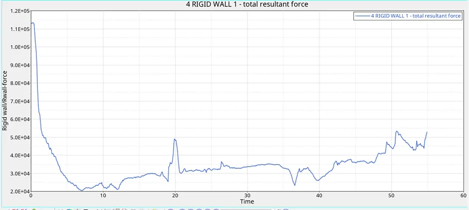
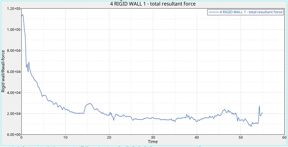
Rigid wall forces: Rigid wall forces are the reactionary forces that are acting on the wall. Initially there was hard contact between the wall and component i.e when the component is just touching the wall at 0ms and about to exert the force the solver did not recorded the force during this phenomenon, it started recording right after the force was applied on the wall at 0ms, because of this we can observe that the reaction forces are very high at starting rather than sharp increase from zero in both the cases. After the initial impact, the forces in the wall are transferred to component, so there was decrease in the R-wall forces in both the cases. After that a rise or dip in the graph can be related to contact area between the component and rigid wall. The higher contact area will cause a raise in the R-wall forces and whenever the rail component bounce back or partially in contact with the wall, this will reduce the magnitude of the R-wall forces and the same can be depicted a dip in the graph. We can see a higher value of R-wall forces at the end of simulation in case-1 compared to case-2 because at the end surface contact was observed between the component and rigid wall. In the second case, there was more realistic deformation, therefore no surface contact was observed at the end of the simulation.
Case-1
Case-2
Contact energy: It is an artificial form of energy that arises when one element tries to exert force on the neighboring element when they are trying to come to contact each other. Initially there was no contact between the component by itself, so the graph started from zero in both the cases and then it increases slowly from there as the deformation increases in both the cases. The element formulation helped to reduce the max value of contact energy compared to case-1.
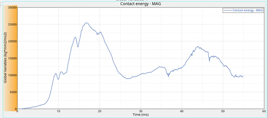
Case-1
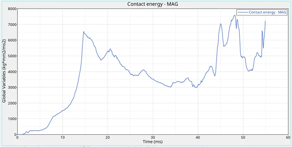
Case-2
Simulations:
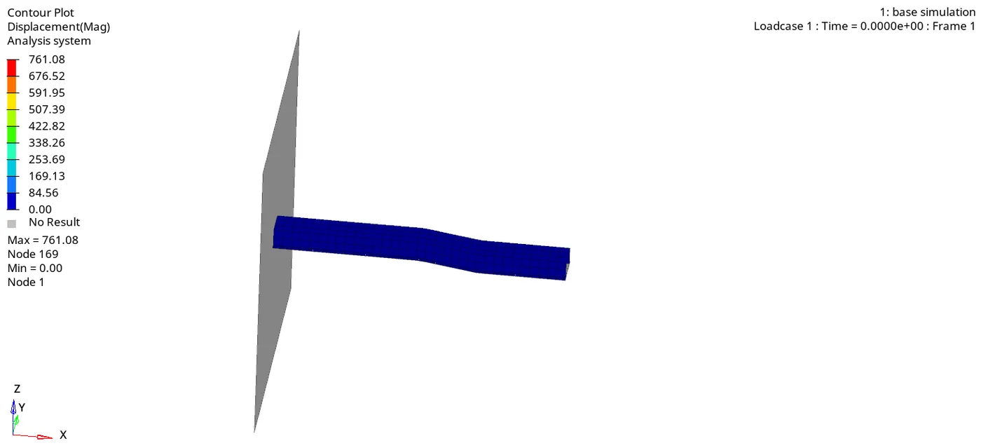
Case-1
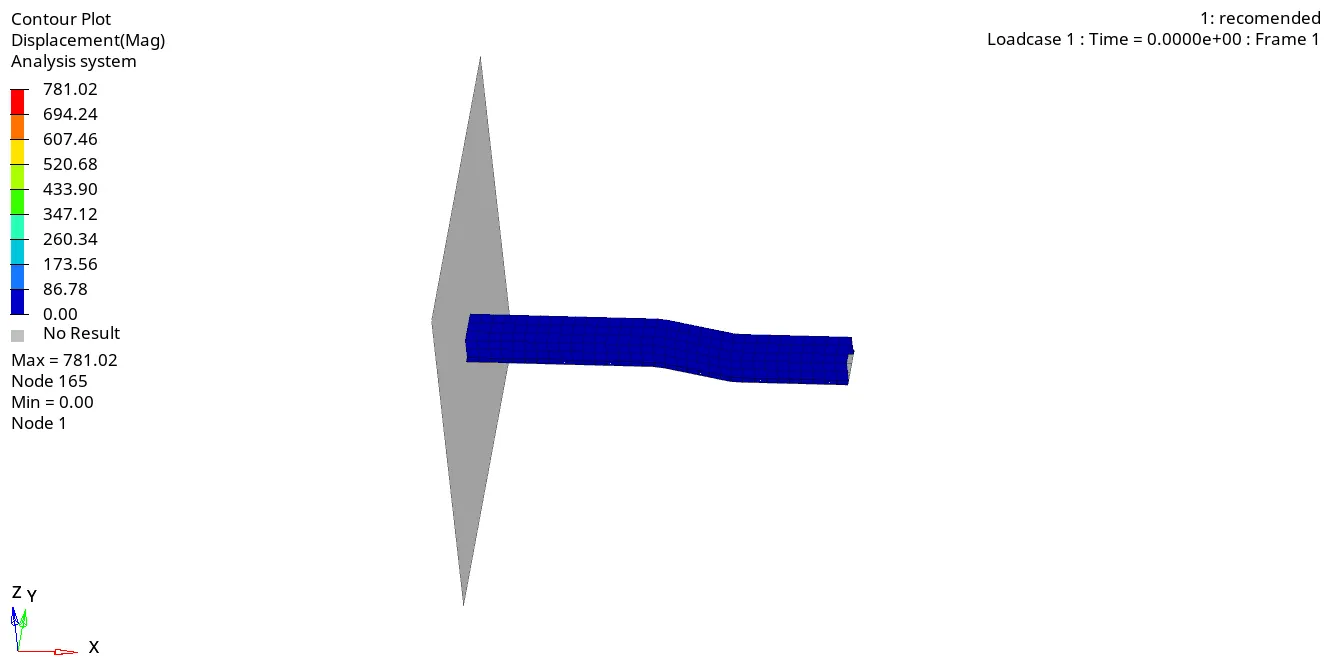
Case-2
From the displacements simulation we can observe that the max displacement in second case was more, this is due to elimination of hourglass energy. All the displacement and strains which are not recorded in case-1 were recorded in case-2 because of the element formulation.
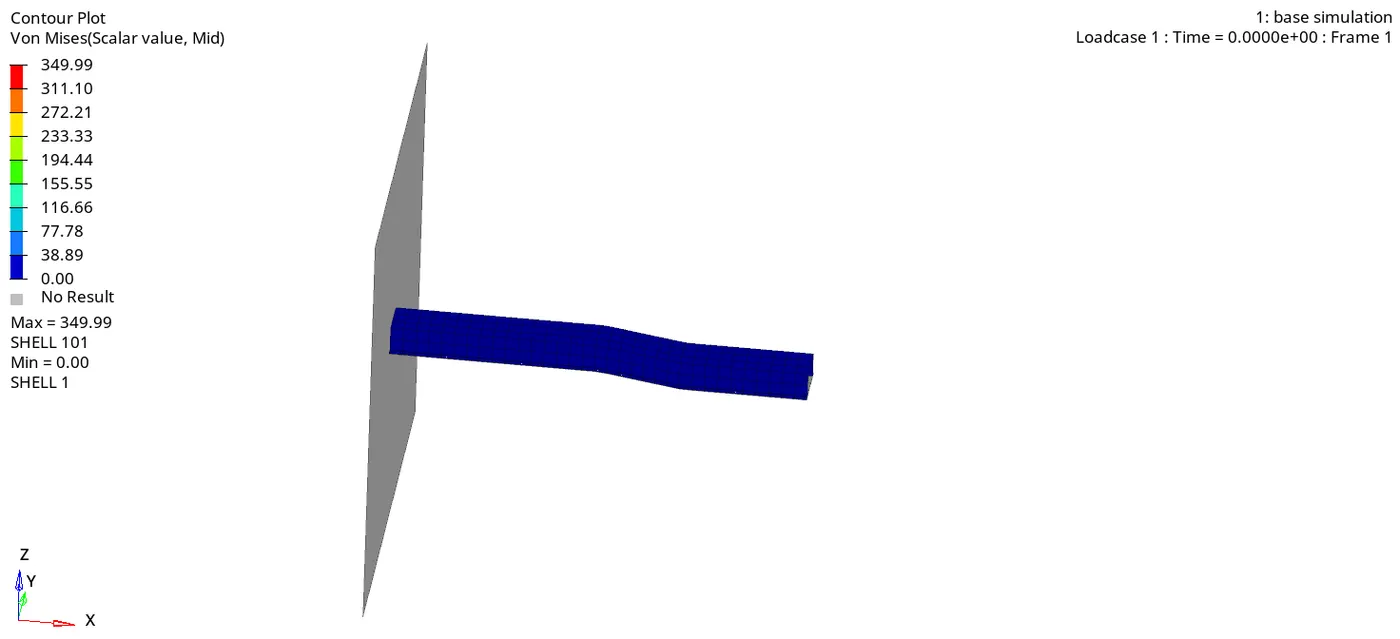
Case-1
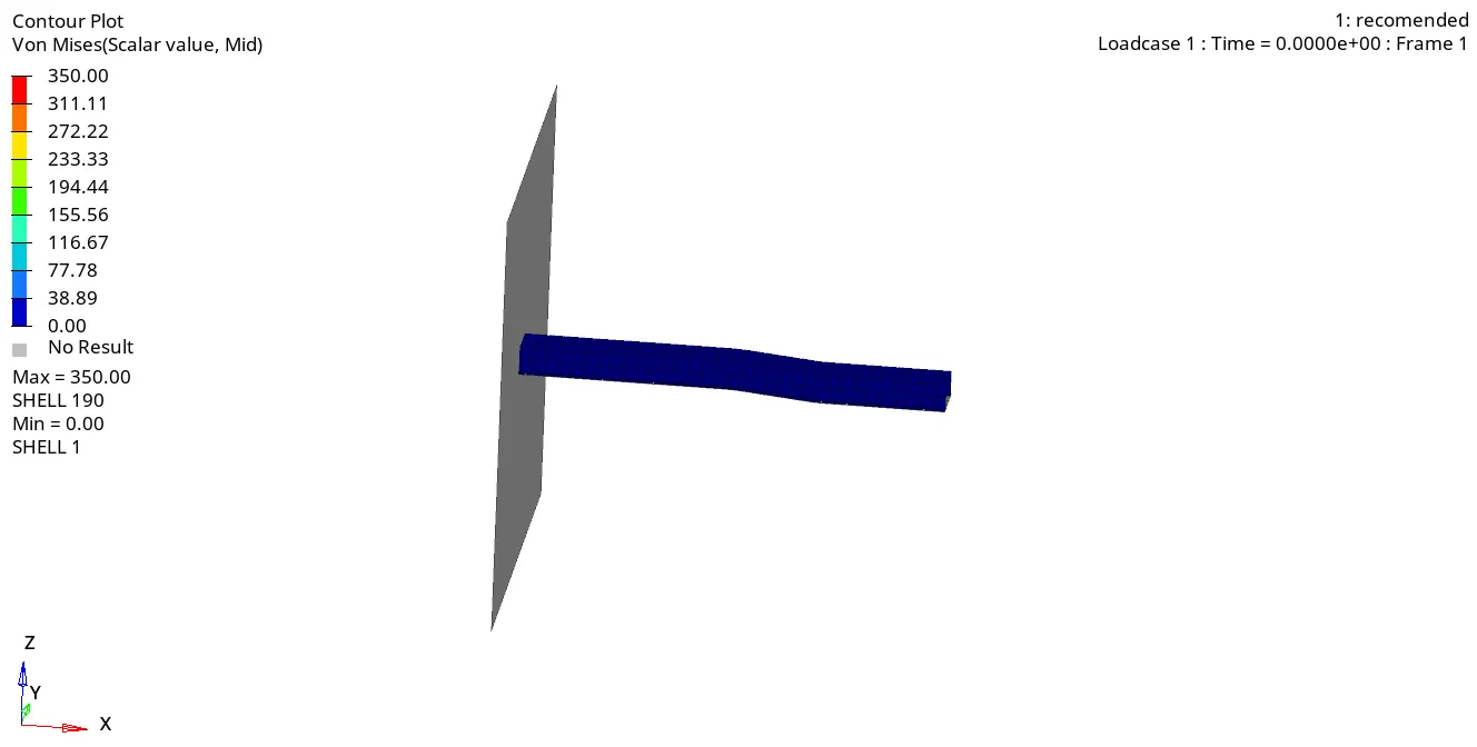
Case-2
We can observe that in both the cases the max von-mises stress are equal. As there is no definite change in force or area in both the cases there are no changes in the stress value.
HOURGLASS:
It is a non-physical form of energy of the system that occurs in first ordered reduced integration elements.
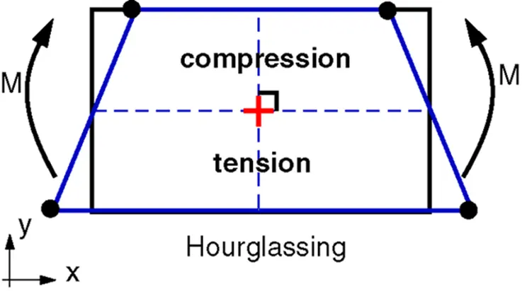
Since single integration point is present right at the transition between compressive and tensile stress zones, we cannot notice change in length of the imaginary lines nor change in angle between the two imaginary lines due to imparted deformation. This results in zero strain deformation modes and can lead to unrealistic results.
Methods to prevent hourglass energy:
· Use of fully integrated points can help us to completely remove the hourglass, but it is computationally costlier and shear locking will take place in the element.
· Perturbation method:
Ø Generally used for Q4 elements.
Ø Damping is applied to control the speed of the deformation.
Ø Damping controls only the speed not the force. So an opposing force is applied on the node to stabilize deformation. This opposing force will produce an artificial energy known as hourglass energy.
Ø Recommended for high velocity and high strain rate problems.
· Physical stabilization method:
Ø Generally used for QEPH elements.
Ø Hourglass is controlled from the material level by adding some stiffness to it.
Ø Very less amount of hour glass energy is needed as it prevents the hourglass effect before it starts.
Ø Recommended for low velocity problems.
CONCLUSIONS:
Ø Simulations were carried out using both default and recommended properties.
Ø Learnt about 2-D element formulations.
Ø Learnt about how to Post process the results using HyperView and Hypergraph 2D.
Ø Learnt about hourglass effect and methods to control the hourglass effect.