Assignment 3-2D Element Formulation Challenge

Assignment 3-2D Element Formulation Challenge

1. Aim

• Using the specified crash beam file, perform simulations with the default and improved shell element properties. Afterwards, analyze and compare the results obtained from both simulations.
• Write a detailed explanation of hourglass energy, its causes and the steps to avoid it.

2. Objective

• Using the crash beam file, Run the base simulation without any modification to element properties by changing the run time to 55 ms and the number of animation steps during simulation to a minimum of 25 and a maximum of 60.
• At the end of the simulation, do the energy error and mass error checks and determine whether the results would be acceptable. If acceptable, Plot rigid wall forces, internal energy, hourglass energy, contact energy, and the total energy of the simulations.
• Change all the shell elements' properties to recommended properties, save this as separate, rad files and run the simulation.
• Do the energy error and mass error checks. Plot the graphs
• Compare the results obtained from both simulations.
• Write a detailed explanation of hourglass energy, its causes and the steps to avoid it.

Improved shell element properties

SL No.	Element Properties	Values	Description
1	Ishell	24	QEPH 4-node shells are the best combination of cost and accuracy.
2	Ismstr	2	Full geometric nonlinearities (default)with possible small strain formulation activation in RADIOSS Engine.
3	Ish3n	2	Standard 3 noded shell (C0)with modification for large rotation(default)
4	N	5	The number of integration points is set to 5 for accuracy bending.
5	Ithick	1	Thickness change is taken into account for accuracy.
6	Iplas	1	Iterative plasticity for good accuracy.

3. Procedure

Default Shell Element Properties

Step 1: Importing the Crash Beam File

Initially, we have to import the file 'Element_Formulation-Shell-3_assignment_0000' to hyper mesh. (Using Solver Deck)

• File >> Import >> Solver Deck >> Browse File location >> Import.

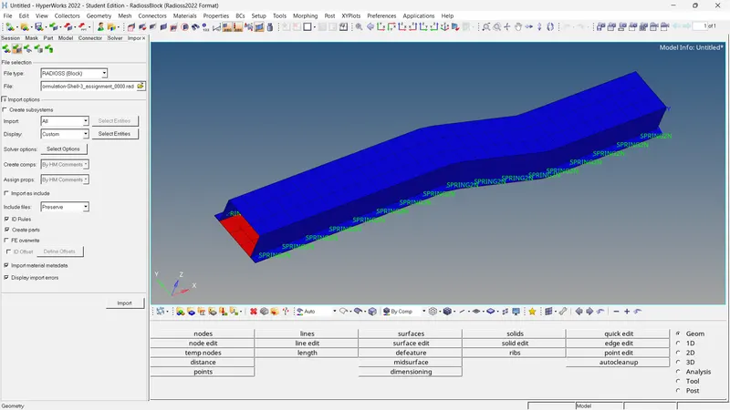
Fig 1: Importing Of Crash Beam File

Step 2: Assigning Run Time and Time-Frequency

Then, we have to assign the run time which is equal to 55ms. The number of animation steps during simulation to a minimum of 25 and a maximum of 60. Let it be the mid value that is equal to 45

So, Run Time = 55ms

No. of Animation Steps = 45

Then, Time-Frequency = Run Time/No. of Animation Steps

= 55/45

= 1.22 ms Per Animation

Assign these values through the solver browser.

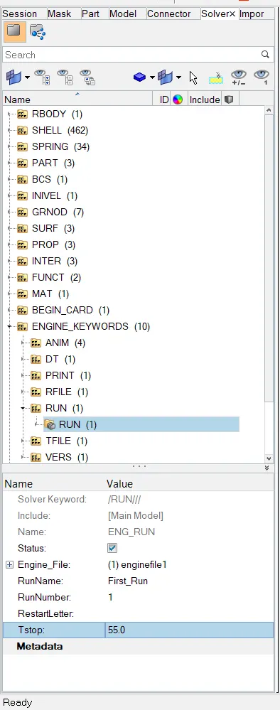
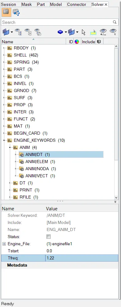
Fig 2: Assigning Run Time and Time-Frequency

For the first scenario, we have to run the simulation using default values (DEF_SHELL), which are pre-assigned. In this model, there are 2 components (Each has a separate Property Card). Simulate as it is.

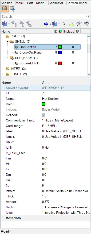
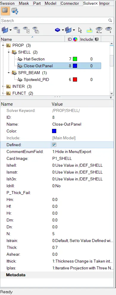
Fig 3: Default Shell Element Properties

Step 3: Simulation And Analysing

Run the simulation by,

• Analysis >> Radioss >> Browse input file location in local directory >> Export Option = All >> Run Option = Analysis >> Run Number = 1 >> Options = '-nt 4' (Choosing Number Of Threads For High and Stable Performance) >> Radioss.

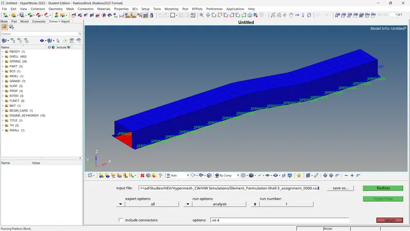
Fig 4: Running Simulation (Default)

After the run, The run summary file (_0001.rad) will load. From that, we can view the output file (_000.out) and inspect the '% Energy Error' and 'Mass Error'. Also, the animation file (.h3d) can be viewed by clicking 'Results'.

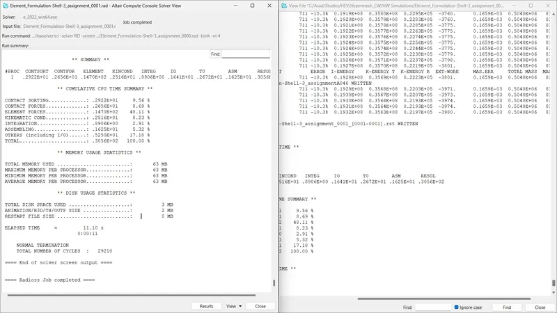
Fig 5: Run Summary File and Output File (Default)

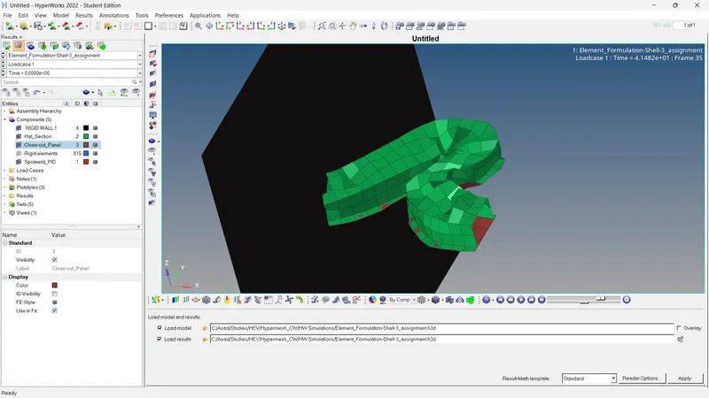
Fig 6: Results using Hyper View(.h3d File) (Default)

• Final % Energy Error = -10.3%
• Final Mass Error = 0.1659E-03

The % energy error is -10.3% which is in the acceptable range (0 to -15%) and mass error stays at constant and is equal to 0.1659E-03. It means there are no issues like model issues. So we can proceed with these results.

Using HyperGraph 2D, we can create a graph that shows their parameters. For this case, we need 'Time Vs Internal Energy / Hourglass Energy / Contact Energy / Total Energy/ Rigid Wall Forces'

• HyperGraph 2D >> Browse File Location (T01 File - Time History File) >> X Axis = Time >> Y Axis = Desired Variable >> Apply >> Ok

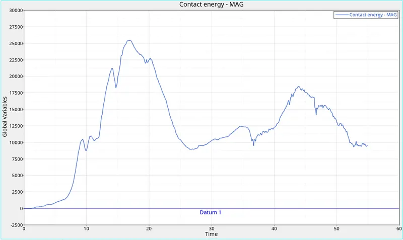
Fig 7: Time Vs Contact Energy (Default)

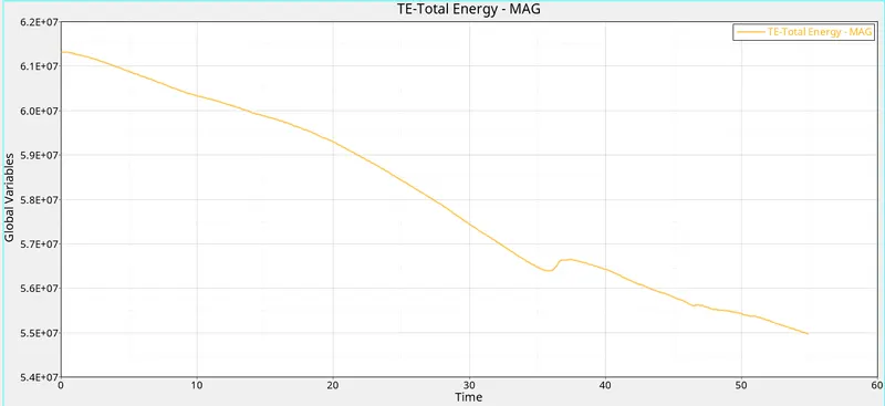
Fig 8: Time Vs Total Energy (Default)

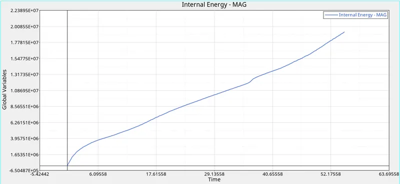
Fig 9: Time Vs Internal Energy (Default)

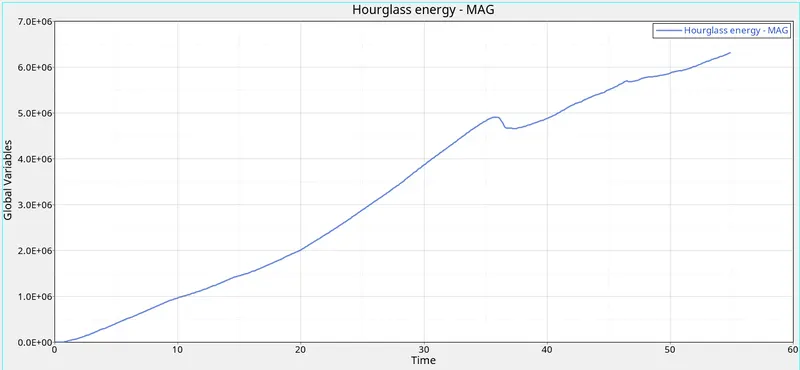
Fig 10: Time Vs Hourglass Energy (Default)

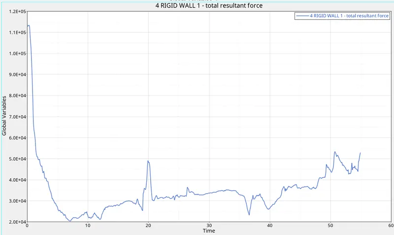
Fig 11: Time Vs Total Resultant Force (Default)

Improved Shell Element Properties

Step 1: Assigning Improved Shell Element Properties

Here we have to assign the given element properties. The run time and time frequency remain the same.

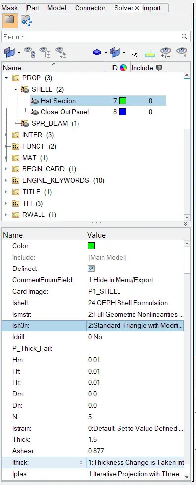
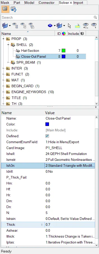
Fig 12: Improved Shell Element Properties

Run The Simulation and Inspect the results and output file

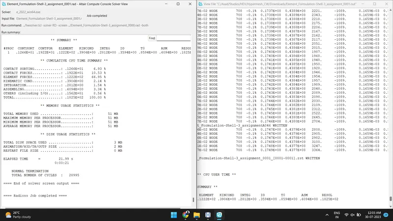
Fig 13: Run Summary File and Output File (Improved)

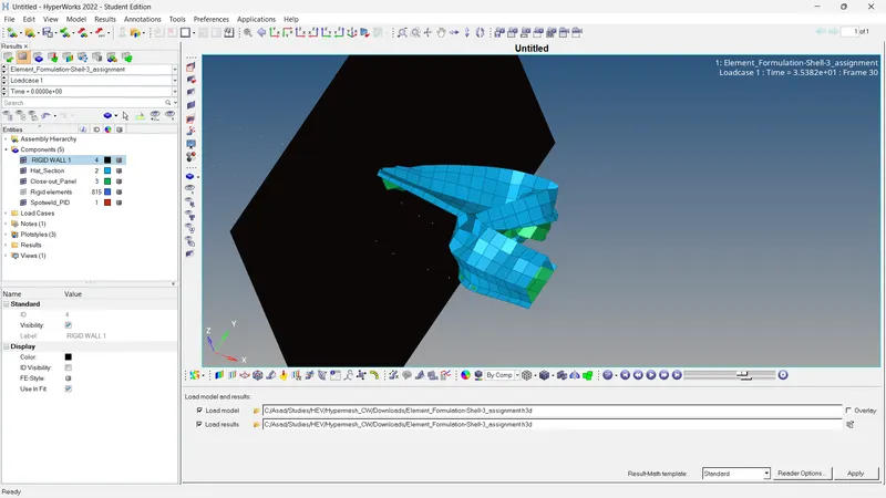
Fig 14: Results using Hyper View(.h3d File) (Improved)

• Final % Energy Error = -0.1%
• Final Mass Error = 0.1659E-03

Both values come under the acceptable range. So we can proceed with the simulation. With HyperGraph 2D, Using the T01 file, plot the necessary graphs and Then compare the results.

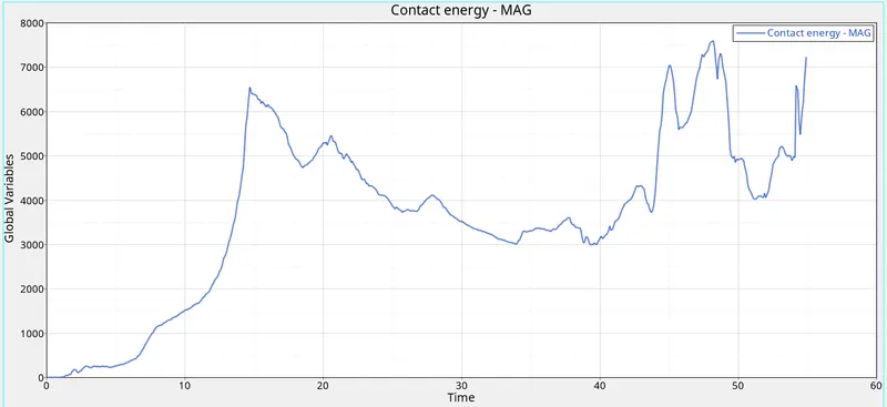
Fig 15: Time Vs Contact Energy (Improved)

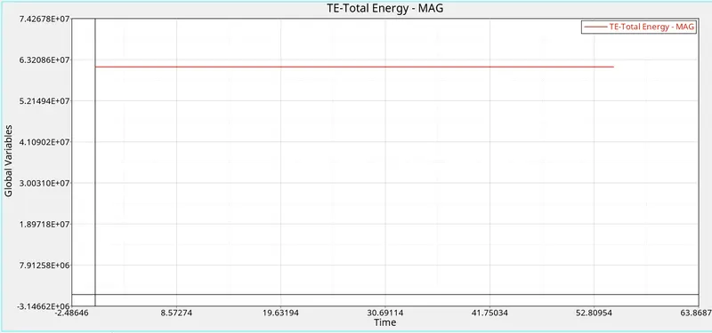
Fig 16: Time Vs Total Energy (Improved)

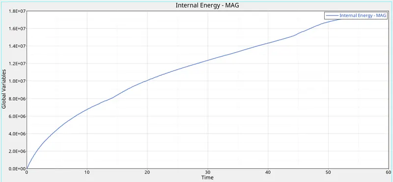
Fig 17: Time Vs Internal Energy (Improved)

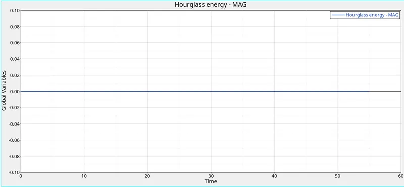
Fig 18: Time Vs Hourglass Energy (Improved)

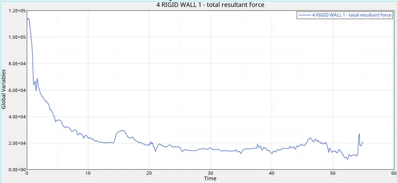
Fig 18: Time Vs Total Resultant Force (Improved)

Comparing Both Results,

Sl No	Results	Default Element Properties (Case 1)	Improved Element Properties (Case 2)
1	% Energy Error	-10.3	-0.1
2	Mass Error	0.1659E-03	0.1659E-03
3	Kinetic Energy	0.3563E+08	0.4377E+08
4	Internal Energy	0.1932E+08	0.1749E+08
5	Total Energy	Decreasing With Time	Almost Constant (~max) With Time
6	Hourglass Energy	Increasing With Time	Minute Increasing (~0) With Time

By analysing the results of both scenarios, The results are more accurate in the simulation with the improved element properties, rather than with the default element properties. We can see that, the energy error is much more high (-10.3%) in the first case. But, when it comes to the second case, the error is almost equal to zero (0.1%). Also, in both cases, Plot 'Time Vs Hourglass Energy' and Plot 'Time Vs Total Energy', are inverse to each other. This means the increase of hourglass energy leads to the decrease of total energy (energy loss) which leads to an increase in %energy error and affects the accuracy of simulation. Also, the mass addition in both cases are same and it concludes mass addition rate and shell element properties are independent of each other.

Hourglass Modes

Definition:

The hourglass modes are non-physical modes of deformation that occur in under-integrated elements (Solid elements with a single integration point or Shell/Tshell elements with a single in-plane integration point) and it does not produce any stress.

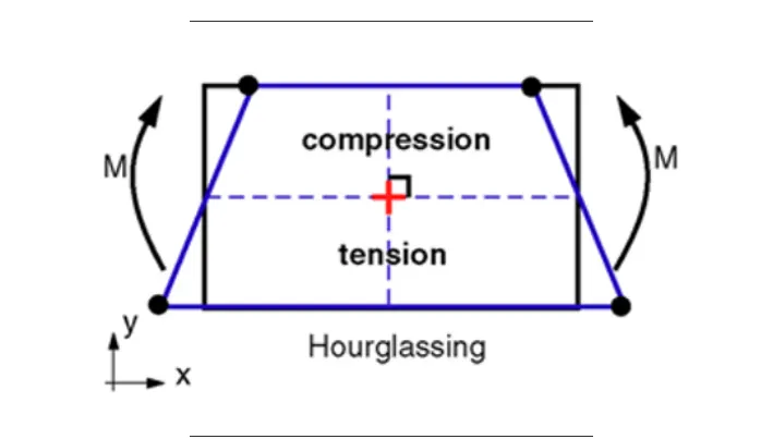
Fig 19: Hourglass mode

To avoid the hourglass mode,

• Using fully integrated solids and shells (More Expensive and Weak for Large Deformations)
• Using Tetrahedrons and Triangles ( Has Locking Tendencies with is bad)
• By applying internal forces to counter hourglass deformation
• By introducing nodal force to counteract hourglass deformation

Methos To Prevent Hourglass Effect

1) Penalty/Perturbation/Viscous Method

• Usined in Q4 element type
• Generate hourglass forces proportional to components of nodal velocity contributing to hourglass modes.
• Inhibits additional hourglassing deformation
• High stability simulation and less accurate results.
• Recommended for high velocity and high strain rate problems.

2) Stiffness Method

• Used in QEPH Elements
• Generate hourglass forces proportional to components of nodal displacement contributing to hourglass modes.
• Able to reduce total accumulated hourglass deformation
• Stability and cost-effective ( Only 15% more expensive than Q4, and almost equal accuracy rate as QBAT)
• Recommended for lower-rate problems.

4. Conclusions

The conclusions are listed below.

Case 1: Default Shell Element Properties

• The element type is 'Q4', (Ishell = 1), which is an under-integrated 4-node element (Belytshko & Tsag). It has one integration point on the surface. It has high stability and the cost is relatively high. This element uses the perturbation method (a.k.a. Penalty Method) for the hourglass energy control.
• The perturbation Method or Penalty Method, is used for the hourglass energy control method, it creates an additional hourglass energy for energy balance. But it also decreases the total energy by time and creates an % energy error causing the accuracy of simulation.
• Less accurate and high stability

Case 2: Improved Shell Element Properties

• The element type is 'QEPH', (Ishell = 24), which is an improved under-integrated 4-node element. It has one integration point on the surface. This element uses the 'Stiffness Method' for the hourglass energy control.
• Unlike the perturbation method, it does not create any additional hourglass energy for the energy balance. It doesn't create any energy error which results in more accurate results.
• Stability and cost-effective

5. Results

• Using the given file, the simulations are performed and conclusions by analysing results and plots from the simulations done in the mentioned scenarios.
• Explained hourglass energy, its causes and prevention methods.