Assignment 3-2D Element Formulation Challenge

Aim - To perform the analysis for the given mesh model with connections. Solve the model in two cases, the effect of hourglass energy and energy error can be determined with the given properties.

Objectives

Import the starter file from the solver deck as shown below and import it to GUI.

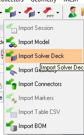
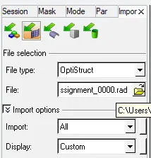
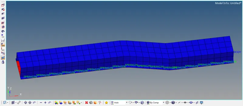
The mesh geometry imported from the solver deck is shown below.

• Here the model is in wireframe mode, Switch to the shaded elements mode as shown below. To switch to shaded mode, Go to Visualization Tab → Shaded Elements and Mesh Lines.

Case I

Comparison of results with base simulation and improved shell element properties

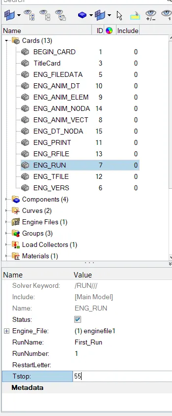
1. Using the crash beam file from the previous assignment, change the run time to 55 ms.

• As per our requirement, we need to change the Tstop Value and Tfrequency Value. To change the values, Go to Model Browser → Control Cards → Edit the values by selecting the appropriate Control Card.

2. Change the number of animation steps during simulation to a minimum of 25 and a maximum of 60.

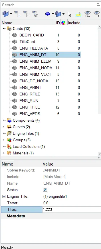
• ANIM_DT [Tfrequency] :
• As per our requirement, the Engine file has to generate between 25 -60 animation files.
• Here I'm taking a maximum value of 45, the solver will create 45 animation files within the termination time.
• Tfrequency = Run Time / Number of Animation Steps
• Tfrequency = 55/45
• Trequency = 1.223
• Now go to the Model Browser → Select appropriate Control Card → ANIM_DT → Enter the Value as 1.223 as shown below

Case I

3. Run the base simulation without any modification to element properties.

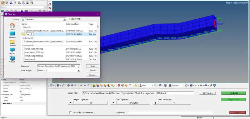
• Go to (Analysis Panel >Radioss>Select the Input File>Save it in Different Folder and Rename it as Case-1>tick box includes connector>option list enter a value -nt_4).
• Check the Include Connectors option if there are any connectors in the model. Thus the connectors will also be taken into account for simulation.
• Type -NT 4 in the options tab, this will result in processing/simulating faster.
• Where NT indicates No of threads,4 indicates assigning of task to 4 cores in the system.

• • The Engine Output File [00001. out] contains the data like
  1. Time Step.
  2. Energy Error.
  3. Mass Error.
  4. Internal Energy Error.
  5. Kinetic Energy Error.
  6. Contact Energy Error.
  • Now check for the Mass Error and Energy Error. The obtained values for Energy Error, Mass Error, Internal Energy Error, Kinetic Energy Error, and Contact Energy Error have been shown below.
  • The Acceptable Energy Error Range is -15% to +5% and the Acceptable Mass Error Range is 0 to 2%.

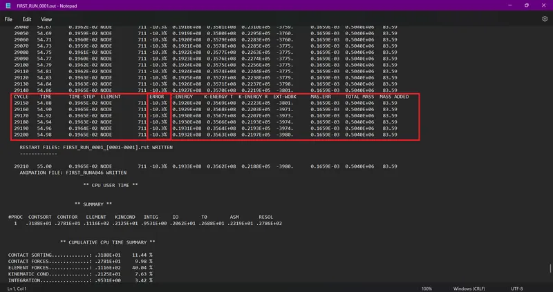
• Maximum Energy Error is= -10.3%.
• Maximum Internal Energy Error = 0.1932 x 10^8 gm^2/s^2.
• Maximum Kinetic Energy Error = 0.3563 x10^8 gm^2/s^2.
• Maximum Mass Error= 0.1659 x 10^-3 g = 1.659 x 10^-4 g.

• Now, these two error values are acceptable, they are not going beyond the standard values.

• After analysis go for the hyper view to run the animation file.

• Apply after importing the file and the mesh model is ready for the animation as below shown.
• After importing the .h3d file into the GUI, Enable the contour. The contour tool creates contour plots of a model graphically visualize the analysis results.
• To enable contour, Go to Results Toolbar → Contour.

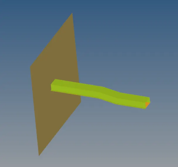
• The mesh model has the all spot weld connections and also has objected to hit as shown below

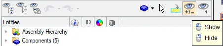
By selecting the hide botton the component will get hide.

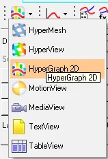
• On the basis of the animation, plot the graph for the various energy for the given component.

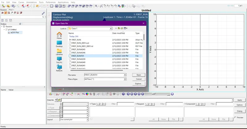
The pages can be split into 2 so that perform the other operations in to account. Use the expand and reduce the window.

Rigid Wall Forces:

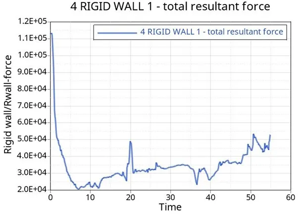
• Total Resultant Force = √f1^2+f2^2.
• Rigid wall forces are the forces that are acting on the rigid wall.
• Here the rigid wall forces are at a higher value in the beginning.
• In beginning, there is no impact in the simulation, But in the graph, the rigid wall forces are at a higher value.
• This is because, the solver didn't record at that time, so the rigid wall force is at a higher value in the beginning.
• When the rail component hits the rigid wall, The rigid wall forces increase from the beginning.
• And it goes on decreasing Because the deformation is happening to the rail component when it hits the rigid wall.

The shared screen is turns in to graph mode as shown in below.

Select the file as the T01 is import in to the GUI and apply it.

By selecting the global varables, select the kinetic energy, inernal energy, total energy, hourglass energy and contact energy can be plotted and selected apply.

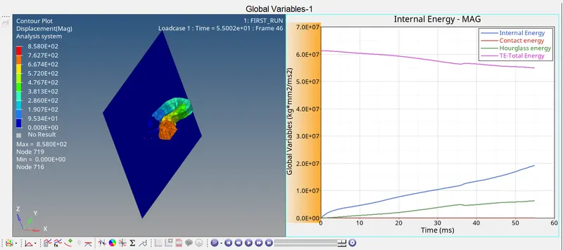
Kinetic energy (KE):

• We know that the formula for kinetic energy is 1÷2mv^2
• The kinetic energy decreases, why because the velocity decreases (The rail component starts to deform, after complete deformation, it will be in rest) when the component comes to a rest, So velocity becomes zero and the kinetic energy decreases.
• So, the kinetic energy is directly proportional to the velocity. That is the reason why, the kinetic energy drops gradually, as shown in the graph below.

Internal energy(U):

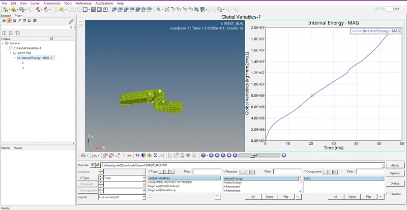
• We know that the formula for internal energy is obtained from the first law of thermodynamics. This depicts the change in internal energy is equal to the difference of the heat transfer into the system(Q) and work(W) done by the system.
• Mathematically, U = Q - W
• let us neglect the heat transfer here because the heat transfer is not calculated by the solver (Because Thermal analysis is not done). Now, Work done (W) is the product of force and displacement. The internal energy depends upon the displacement mush here. In the beginning, there is no displacement within the component, that’s why the internal energy starts from zero(origin). when it is subject to acceleration there will be a displacement. As the displacement increases, the internal energy increases, that’s why there is a raise internal energy curve, as shown in the graph below.

Contact Energy:

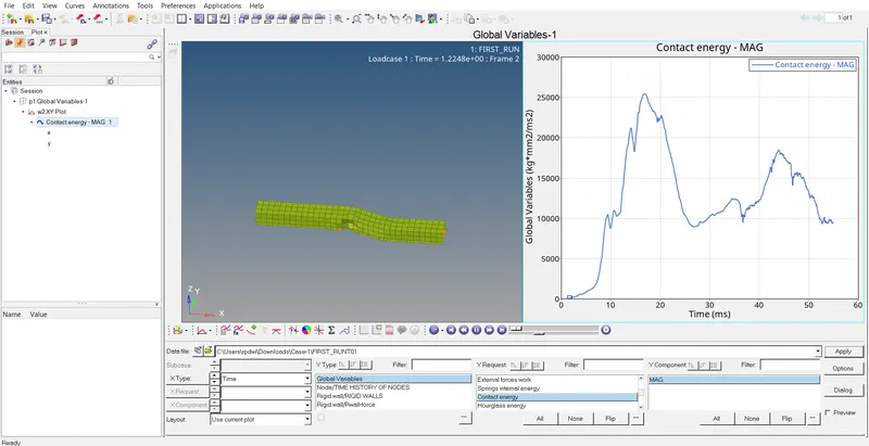
• Here the contact energy starts from origin, Cause the rail component is in the initial condition.
• Initially, there is no contact between the rail component and rigid wall.
• There is also no deformation initially, But when the component goes and hits on the rigid wall, The contact energy starts increasing.
• When the deformation or displacement happens to the component, the contact energy increases, causing the crash tube or rail component to come within contact with the rigid wall. So the contact energy goes on increasing.

Hourglass energy:

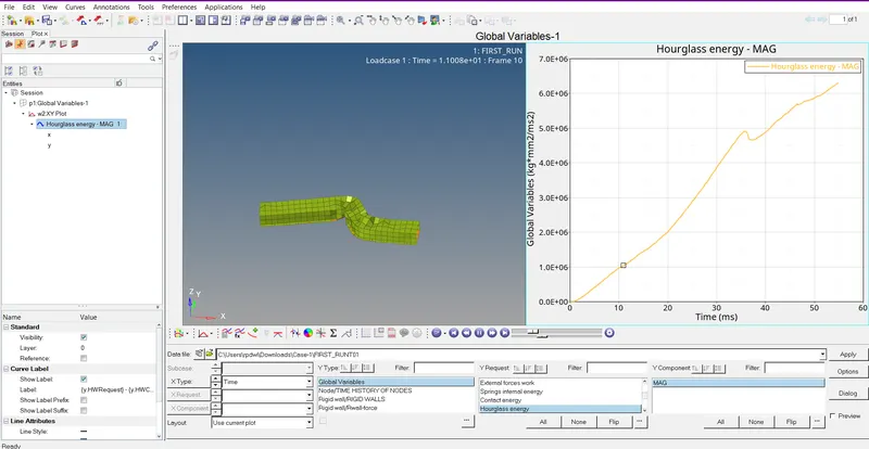
• Here the hourglass energy is starting from the origin because the recommended parameters have not been specified.
• The hourglass energy goes on increasing, Because to balance the rest of the energies, An artificial energy is required, that is called hourglass energy and that's the reason why hourglass energy goes on increasing from its origin. A lot of hourglass energy is needed, So it goes on increasing.

Total energy:

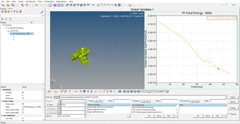
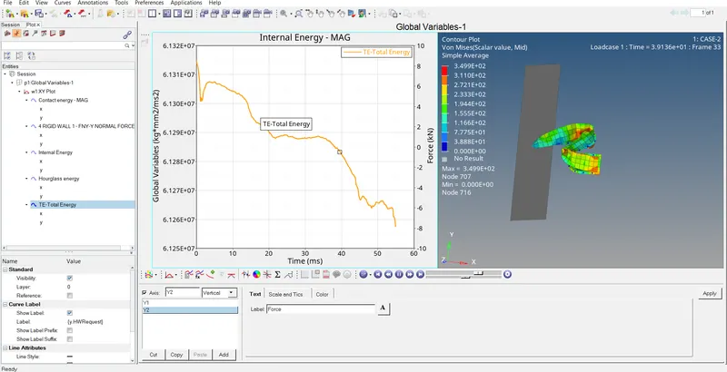
• We know that Total energy is the sum of kinetic energy and potential energy. As there is no potential energy plotted here, the kinetic energy is taken into account. The total energy is directly proportional to kinetic energy. As the kinetic energy decreases, the total energy also decreases

Case 2 - With Assigning the Recommended Parameters in the Property

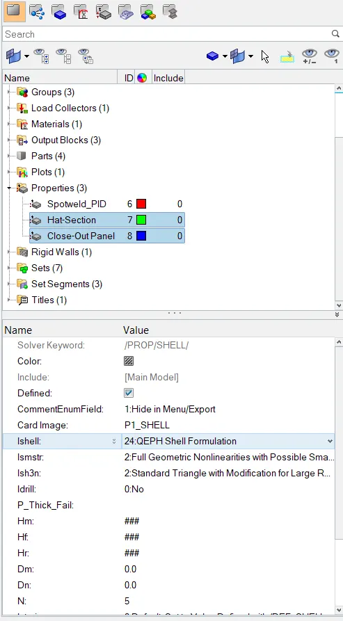
• Now enter the recommended parameters in properties called Hat-Section, Close-Out-Section which is given in the question.
• The recommended parameters have been entered in the properties as shown below.

Parameters		Comment
Ishell =24		QEPH 4 nodes shells are best combination of cost and accuracy.
Ismstr=2		Full geometric nonlinearities (default)with possible small strain formulation activation in RADIOSS Engine.
Ish3n=2		Standard 3 noded shell (C0)with modification for large rotation(default)
N=5		Number of integration points set to 5 for accuracy bending.
Ithick=1		Thickness change is taken into account for accuracy.
Iplas=1		Iterative plasticity for good accuracy.

Similarly, follow the same process and do the same as what we have done for Case 1

• Now run the simulation for Case 2.
• Save the Case-2 in another location to have animation files and engine output files etc., and rename it as Case-2.
• 

case the energt error has been shown the -0.1% so, its acceptable. Its due to the assigning the recomanded properties to the perticular case.

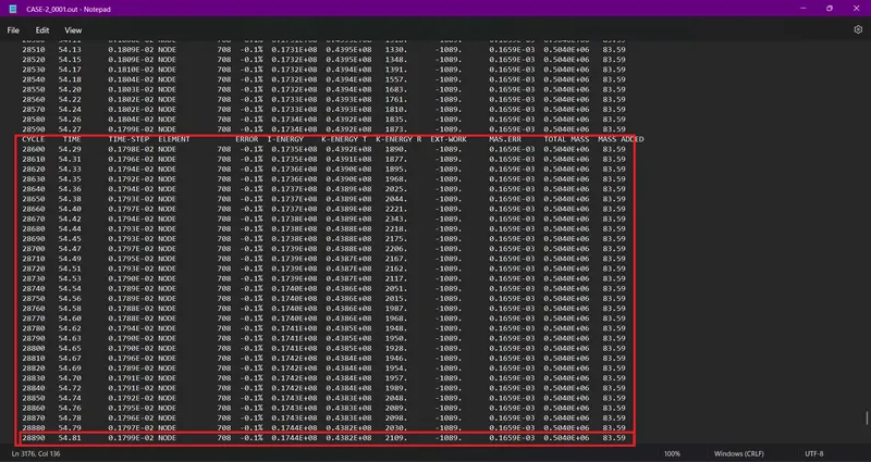
• Now go and open the Engine Output file to check whether there is an improvement or not.
• There is an improvement when compared to the values obtained from Case 1.
• Here the Energy and Mass Error-values are acceptable and start to run the simulation.
• In any new window switch to the hyperview and then load the .h3d file. Now run the simulation and in the result type switch to the Von misses stress as shown in below.
• Now plot the graphs for the energies. To see the changes in the results with respect to case-1. Plot the graphs for all the energies.
• Here the graph has been plotted for the rigid wall forces which are shown below. Similarly, plot the graphs for all the energies.

Here there is a little bit of improvement after assigning the recommended shell parameters when compared to case-1

Contact energy - The energy has beeen generating from the contact between 2 surfaces and by comparing to this it has been negligible.

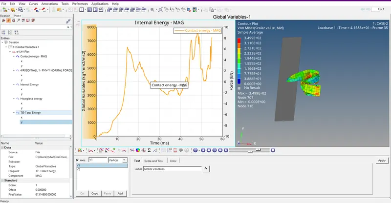
Kinetic Energy- In the garaph shown the kinetic energy is high initially and kanetic energy is decreases w.r.t time. The kinetic energy is directly proportional to the mass and velocity.

As the velocity decreases the kinetic energy also decrease at time period of 55 ms. The effect of the K.E in graph shown in below. For kinetic energy the parameter has been

already assined

K.E= 1/2mv^2

• 

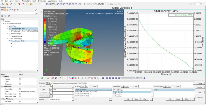
Rigid wall-force-Here the graph has been plotted for the rigid wall forces which are shown below. Similarly, plot the graphs for all the energies

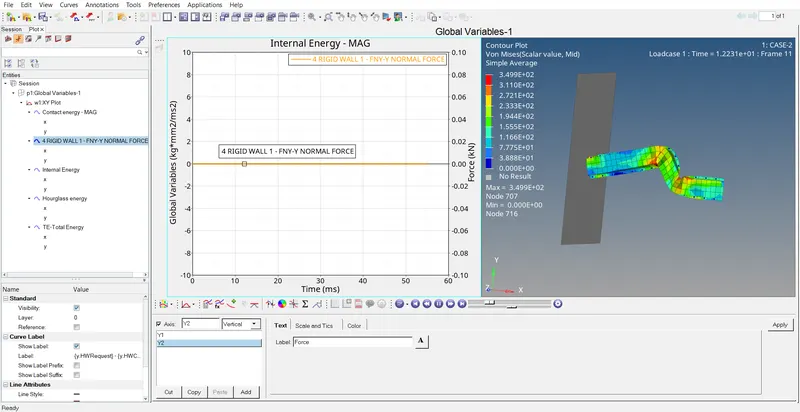
Internal energy-For the internal energy there is initially no deformantion in the component so, in the graph has been started from origine.

Gradually there is change in the deformantion in the model so graph has been increases from origine to some height w.r.t time.

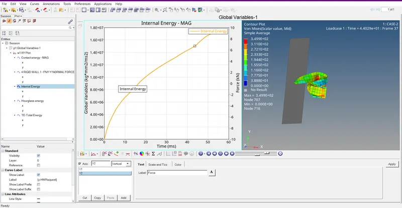
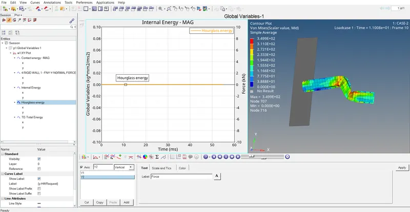
Hourglass energy:

• Here there is a little bit of improvement in all the energies when compared to case-1.
• Now plot the graph for the hourglass energy to see the result, whether there is any improvement in hourglass energy or not.
• Here hourglass energy is constant,Why because the recommended parameter Ishell">IshellIshell=24 [QEPH 4 noded shell].
• It will be having 4 nodes in the element,So hourglass won't happen,It will be constant.
• In previous case,It was under integrated node,So there was hourglass deformation.
• The graphs plotted for Case 2 is as shown below. Here in the case 2 graphs there is no great changes except in the hourglass energy.

• Total energy- Total energy has been taking count of all resultant energies and it has been starting from where the error energy will occur. The energy error will be in the range of -15% to 5%. Particularly for this

Comparison of Case 1 & Case 2:

S.No	Characteristic	Case-1	Case-2
1.	Maximum Energy Error	-10.3%	-0.1%
2.	Maximum Kinetic Energy	0.3563E+08	0.4377E+08
3.	Maximum Internal Energy	0.1932E+08	0.1749E+08
4.	Total Energy	Total Energy Increases and Slightly Decreases due to Energy Error	Total Energy Remains Constant.
5.	Hourglass Energy	Hourglass Energy Increases due to the balance all the energies.	Hourglass Energy Remains Constant due to Recommended Shell Parameter.
6	Contact Energy	The contact energy will produces with mating the 2 objects is negligible	The contact energy will produces with mating the 2 object is less.
7	Regidwall forces	Initially with high force will apply after it becomes gradually decreasing.	Initially with high force will apply after it becomes gradually decreasing. At finally the model is hit with object create with increasing force as shown in the graph

RESULT:

• Hence the simulation has been runned without assigning recommended shell parameters.
• Hence the simulation has been runned with assigning recommended shell parameters.
• The graphs have been plotted for case-1 and case-2 successfully.
• While comparing Case-1 and Case-2,Case-2 is effective,Cause there is no hourglass deformation.

CONCLUSION:

• I conclude that Case-2 with assigning recommended shell parameters is effective.
• In this Challenge the learning outcomes are the procedures of how

1. to run a simulation with and without assigning shell parameters.
2. to do postprocessing (Plotting the graphs for the various parameters).
3. to understand the curves that are increasing and decreasing in the graphs.
4. to compare the obtained values with the various parameters.