Assignment 3-2D Element Formulation Challenge
Objectives:
The primary objective of this assignment is to compare two simulations with different shell element properties. The comparison would be between the one with default properties and one with the following properties.
| Parameters | Comment | |
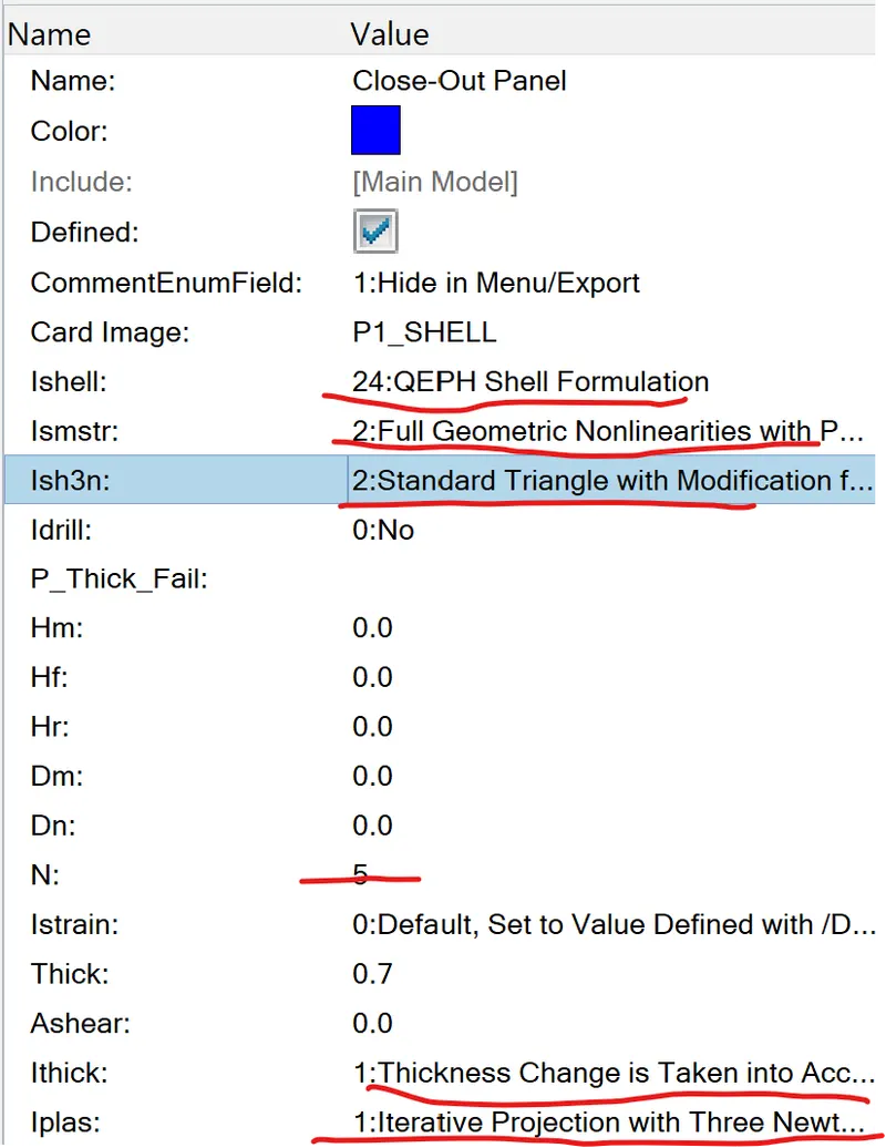
Ishell =24 | QEPH 4 nodes shells are best combination of cost and accuracy. | |
Ismstr=2 | Full geometric nonlinearities (default)with possible small strain formulation activation in RADIOSS Engine. | |
Ish3n=2 | Standard 3 noded shell (C0)with modification for large rotation(default) | |
| N=5 | Number of integration points set to 5 for accuracy bending. | |
Ithick=1 | Thickness change is taken into account for accuracy. | |
Iplas=1 | Iterative plasticity for good accuracy. |
Questions:
1.Using the crash beam file from the previous assignment, change the run time to 55 ms.
2. Change the number of animation steps during simulation to a minimum of 25 and maximum of 60.
3. Run the base simulation without any modification to element properties.
4. At the end of the simulation, do the energy error and mass error checks and determine whether results would be acceptable.
5. If acceptable, Plot rigid wall forces, internal energy, hourglass energy, contact energy, total energy of the simulations.
6. Change all the shell elements properties to recommended properties, save this as separate, rad files and run the simulation.
7. Follow steps 5 and 6.
8. Create a brief report comparing all the results from steps 5 and 6 for both simulations.
9. Comment whether there is any change in the results and why there is any change in the result.
THEORY
The following properties are changed for case 2.
Ishell">Ishell: This is the element formulation for 4-noded shells
Ismstr">Ismstr: This property is to specify small or large strain formulation
Ish3n">Ish3n: This is the element formulation for 3-noded shells
N: The number of integration points through the thickness
Iplas">Iplas: Method for calculating post-yield strains
Ithick">Ithick: Property that decides if the thickness is constant or to consider if element thins.
About Hourglass deformation:
Hourglass is basically a kind of deformation that is produced during the simulation in certain shell elements that have not been integrated appropriately. As a result, stress is not produced in these elements and this reduces the accuracy and true response of the structure during the simulation. This effectively results in incorrect displacement results with unrealistic representations of the simulated part.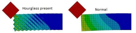
How to reduce hourglass?
There are two ways to control hourglass formation. One is via Perturbation method and the other is through Physical Stabilization. It is important to deploy the right method based on the conditions of the simulation.
Perturbation is deployed by Q4 elements (Ishell">Ishell= 1, 2, 3, 4) and involves introducing an opposing force to stabilize whichever node it detects potential hourglass formations. This opposing force produces energy and that's known as 'hourglass energy'. As mentioned before, this method fails for large rotation and elastic loading-unloading cycles. In addition to that, it uses a simple under integrated method and this takes lesser time and computational power but that comes at the cost of accuracy.
This is why the Physical Stabilization method is the best method since it can be used in any case. This method is deployed by QEPH elements (Ishell">Ishell = 24) and involves introducing an artificial stiffness. As a result, shell elements are controlled from a material level and in addition to that, they use an improved under-integrated method that provides the best compromise between computational cost and accuracy.
Procedure:
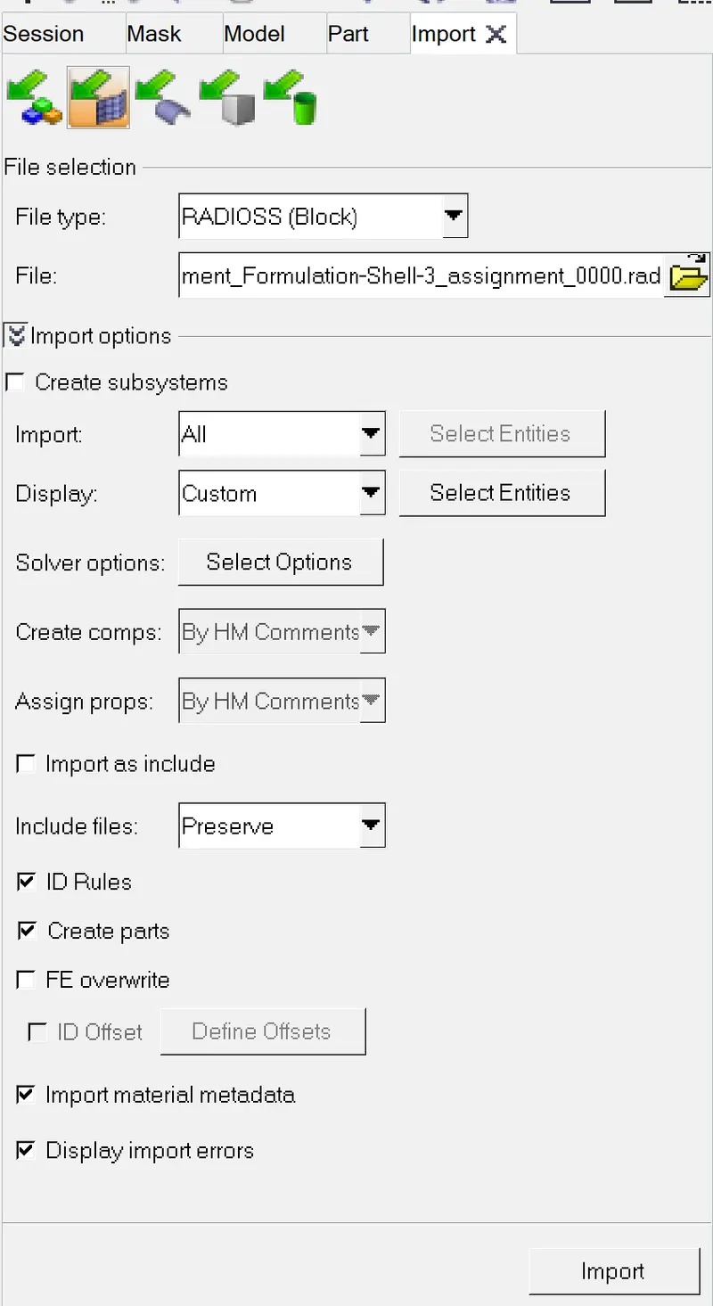
1. first we have to import the file. The importing of the file takes place as import > solver deck. select the file which is the starter file which is in the form of 0000.rad file.
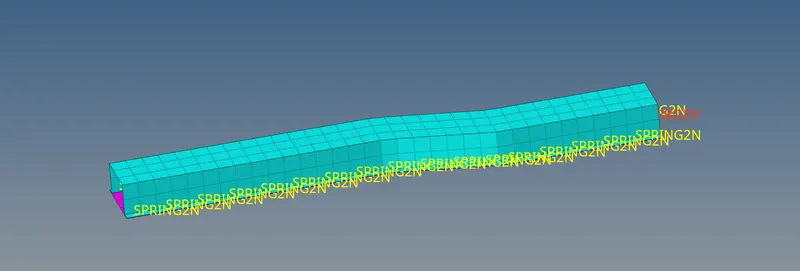
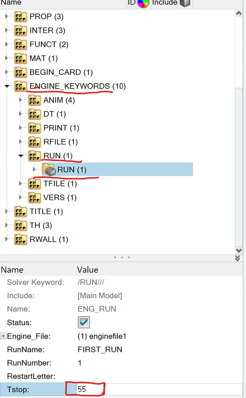
The first question is to change the run time to 55ms for that we have already imported the model next is to change the run time. For the changing the run the we have to go for solver > ENGINE_KEYWORDS > RUN >ENG_RUN . After that change the Tstop = 55.
2. The next questions is to change the number of animations by using a same command that is solver > ENGINE_RUN >ANIM> ANIM DT. After that change the required attrubutes.
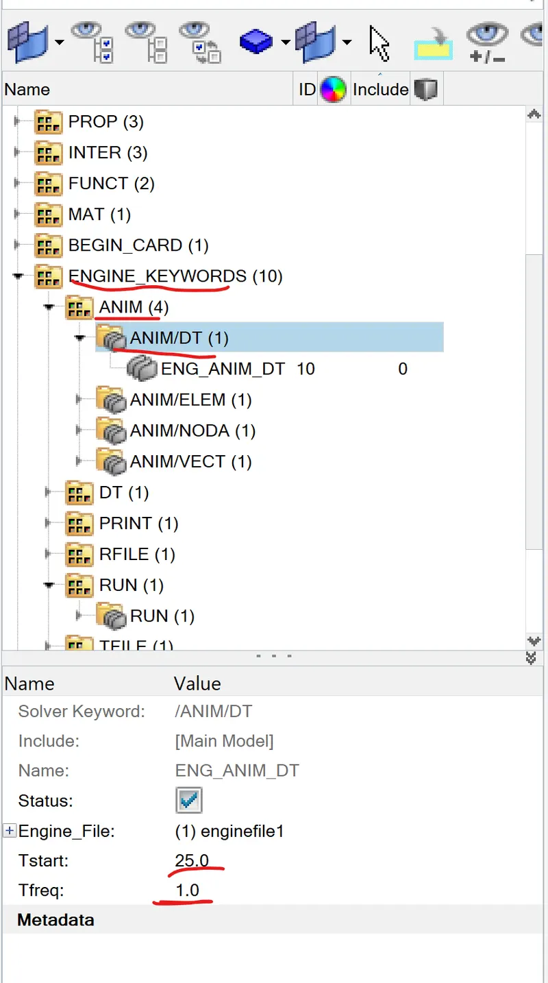
The value of time start is set to 25 and T freq is set to 1.
3. Next requirement is to run the base simulation. For that, we need to save the current file with edited parameters. This can be carried out via the analysis process.
For this, we can go to the 'Analysis' section from the bottom panel.
There, we can select RADIOSS.
In the next section, we are given the option to save the file before running it in the solver. We can go ahead and give it a different name from the base file to avoid confusion. Clicking 'save as' lets us do that.

After saving we need run before running we have to include connectors and options we have to write -nt 4 because to increase the processing power of the solver (as in to use all 4 cores). After that, we can click 'Radioss' to activate the solver and it processes the file. We get a solver window that tells us what's going on in the process. It runs for several seconds before finishing and letting us know about completion.
After the completion, we get another window that shows the completion of the analysis. The next is to View the results by changing the hypermesh to hyperview. The changing takes place by using client selectors > Hyperview.
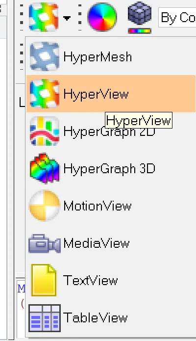
Entering to the Hyperview we have to select the load model and load result which on the same directory that is .h3d file.
After selecting the file we have to apply.

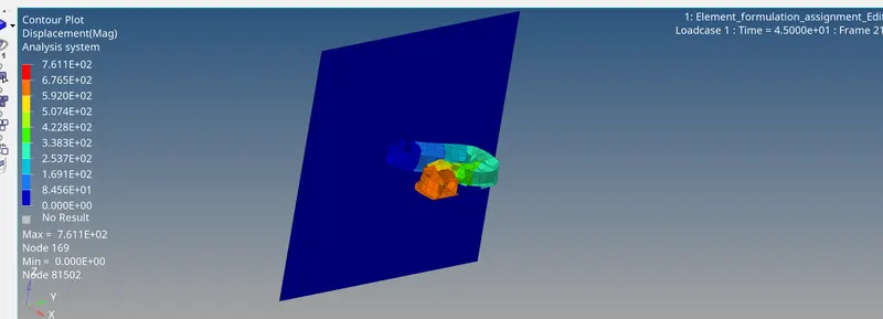
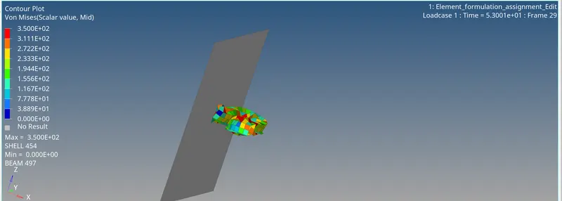
4. Next step is to carry out energy error and mass error checks and this is done by analyzing the RADIOSS engine output file. This can be accessed from the same directory as the starter and engine files and is denoted by the '.out' extension. We need to check the file that contains '_0001.out' by using any text editor.
On opening the file and scrolling down to the end, we can see the final energy and mass error values.
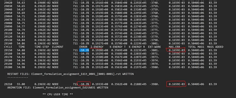
The final energy error is -10.3%, which is less than the threshold of -15% and is acceptable. Acceptable energy error values are supposed to be between -15% and 10%. The closer to 0 it is, the better.
5. With the energy and mass errors deemed acceptable, we can go ahead and plot the graphs. For this, we shall be using the Hypergraph client. We can switch to it using the same client selector option in the toolbar.
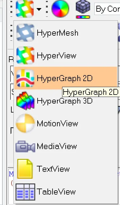
In the Hypergraph section, we are met with a graph and in the panel below, we are to input a file. For this, we will be using the result file generated by the RADIOSS solver (also known as the 'T01 file'). This file is available in the same directory as the starter, engine and animation files. The file name ends with 'T01'.

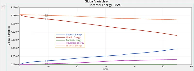
First, we can take a look at the energy graphs (internal energy, hourglass energy, contact energy, kinetic energy and total energy)
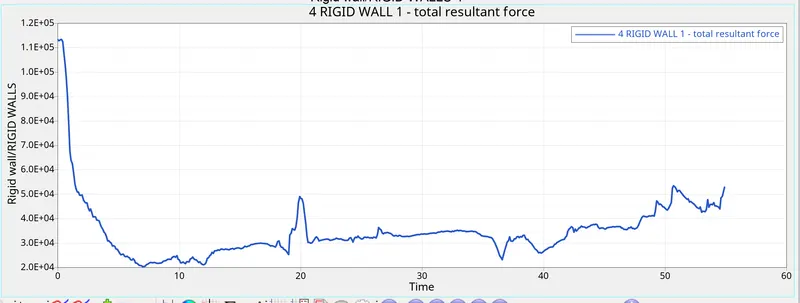
Now we have to plot the rigid wall forces.
6. For this question, we are to carry out a simulation for a new case with the recommended shell element properties. We can repeat the process of importing the original solver deck file and change the values in the solver tab.
After that, we can move to the model tab and go to the properties submenu. The shell properties of the model's components are to be changed so we need to select each of 'Hat-Section' and 'Close-Out Panel' one-by-one and change the values in the property window below as shown.
Next is to go for the analysis > Radioss > save the file with different name.
After that, we can switch to Hyperview to generate the simulation. Like last time, we need to pick the h3d file of this case and click apply.
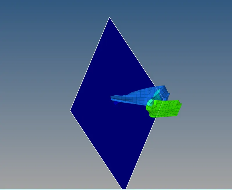
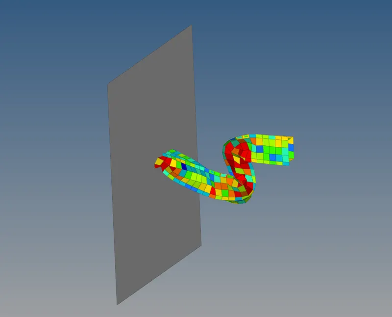
The above figure shows the displacement and the von misses animation.
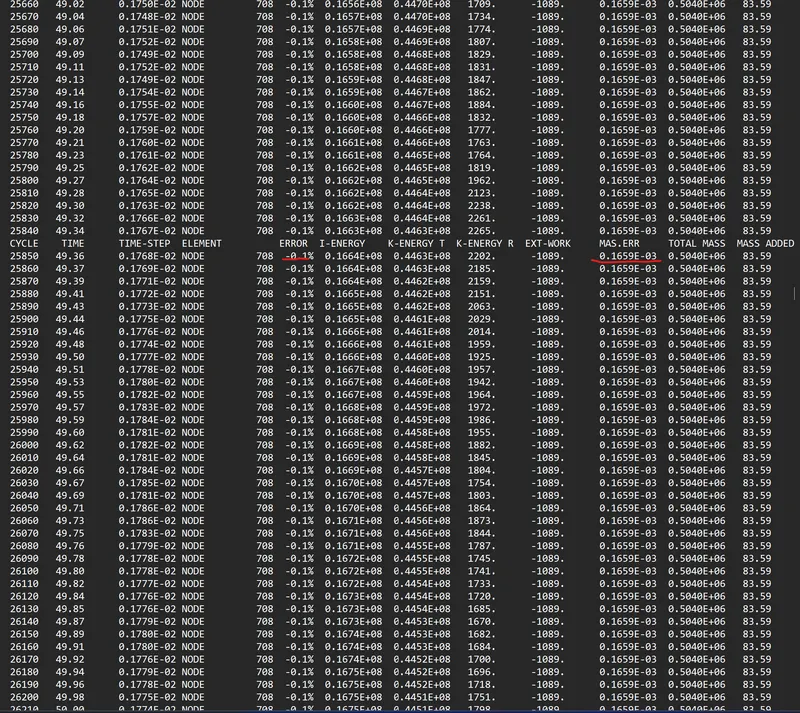
7. Having generated the simulation, we can go ahead and carry out energy and mass error checks, again using this particular simulation's RADIOSS output file. This can be accessed from the same directory as the starter and engine files of this simulation and is denoted by the '.out' extension. We need to check the file that contains '_0001.out' by using any text editor.
Now we can generate the graphs by switching to Hypergraph and selecting this simulation's T01 file. Firstly, the energy graph:
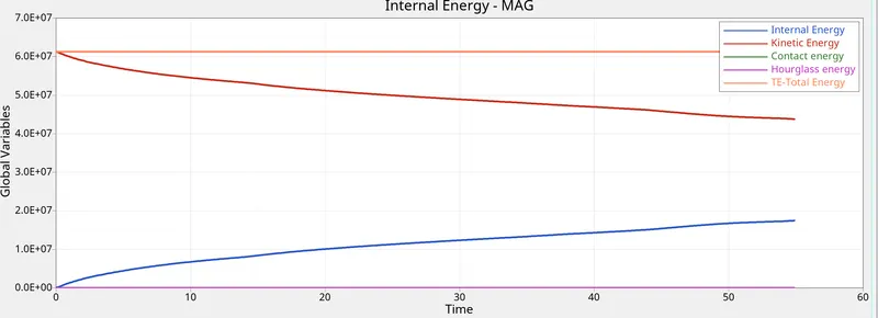
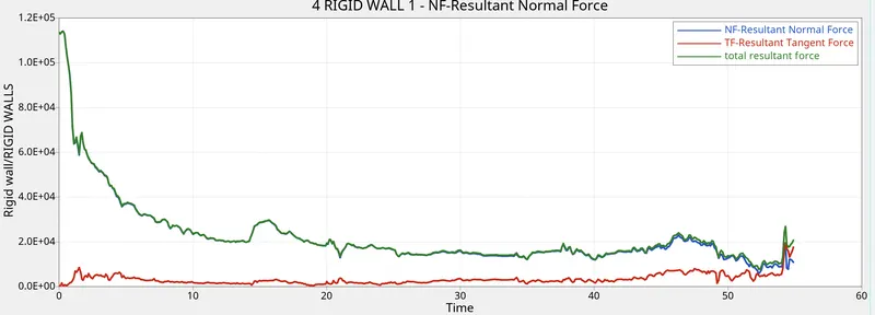
The obvious difference in both simulations is the reduction in hourglass energy. The introduction of QEPH shell formulation (Ishell">Ishell = 24) in the second case, provides an artificial stiffness to the shell elements and helps counter hourglass formation.
A result of hourglass reduction is the more 'natural' looking simulation in the second case, with less crumpling.
Overall, there have been some obvious differences in results. To summarize:
| Attribute | Base Simulation | Simulation with recommended properties |
| Energy Error | -10.3% which is acceptable (average result) | -0.1% A good number since it's almost 0. |
| Total energy | Total energy reduces over time due to the introduction of hourglass energy | Total energy remains constant since there is barely any hourglass energy |
| Hourglass Energy | Hourglass Energy increases over time | Hourglass energy remains zero |
RESULTS
Two simulations were carried out on the same crush beam using different shell element formulation properties.
Comparing the results of both cases, it can easily be figured out that there is a big difference in the values of hourglass energy, internal energy and rigid wall forces.
Also, the amount and nature of deformation of the 2nd case are much higher and different than the first case. This deformation is more practical than the base simulation. This improvement is definitely due to changes in the material card and its element properties.
It was established that using the recommended settings helped reduced hourglass formation drastically due to the introduction of the physical stabilization method that is deployed by QEPH elements.