Assignment 3-2D Element Formulation Challenge
Title : Various Formulation Methods for 2D Elements
Objective : To understand the various 2D element properties that affect the accuracy and cost of the simulation.
Theory :
An element undergoes through a large deformations in the crash analysis application. This leads to various accuracy issues of the element. As most of the part of the car are constructed using shell elements it is important to understand the various properties that are supposed to be set with keeping a good balance of accuracy and the cost of the simulation. In this work the discussion is kept limited to 2D elements. Following are some of the issues that occur in the element.
i. Hourglass
Hourglass is the deformation in the element that is occured due to the rapid force on the element. But the strain energy is not recorded for that element, i.e no stress value is recorded eventually leading loss of energy from the simulation. Hence by controlling the hourglass, an external energy is added into the simulation which is named as Hourglass Energy. If the user adds this energy with Kinetic and Internal Energy, the balance of energies might be explained properly.
There are two main ways to control the Hourglass,
a. Perturbation Method (Viscous Damping) : After detecting the hourglass some damping is applied which eventually stabilizes the deformation and controlling the deformation.
b. Physical Stabilization Method (Stiffness Method) : Stiffness is added in this method at the material level. This addition makes the element stiff and prevents the non physical deformation. As in this method the control is done well before the amount of energy required is less and eventually lower hourglass energy is seen compared to viscous method.
In defining the property to shell element i.e 3 node or 4 node shell element PROP/SHELL shell property is used. Following are the fields required to define a shell property card.
Ishell : This option describes the shell element formulation. Available options are 0 (default shell card),1(Default if Def_shell card is not defined),2 (Q4 visco elastic),3 (Q4 elasto plastic),4 (Q4 improved),12 (QBAT shell),24 (QEPH shell ). 1 to 4 are reduced integration elements, 12 is full integration element and 24 is improved under intergrated.
Ismstr : Shell small strain formulation. 0 uses value from DEF card. 1 to start the small strain formulation from time 0. The value 2 is for high deformation problems i.e for consideration of the geometric non linearities. So in this case the strain is calculated at the instantaneous size of the element and not using the initial value of the element. This is the default value for the small strain formulation. The usage of this is to be controlled by the user as in case of very large values of deformation the time step may decrease and affect the stability and in this case the user must switch to value 1.
Ish3n : This formulation is for 3 noded element. They have only one integration point and no hourglass as the element has only 3 node and the node cannot go out of the plane.
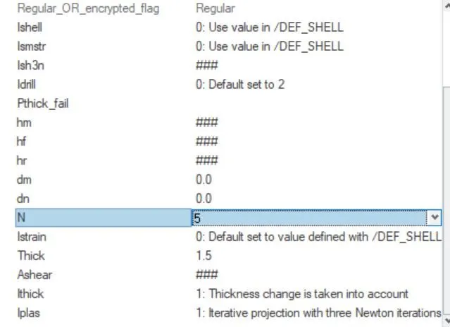
N : Number of integration points through the thickness. General standard value is 5.
Ithick : In this feature the thickness change effect is considered. The value 1 states that the change in the thickness should be taken into account for calculation of results. The value 2 states that the thickness of the element remains same over entire simulation time. It is recommended to keep the value to 2 as no cost is affected with this.
Iplas : This option takes care of switching to plastic region. It is recommened to keep the value 1 i.e the iterative projection with newton iterations as the value of strain is updated throught the thickness and new thickness is computed and the results are passed on the surface.
In this work the effect of this features needs to be studied using a crash tube which crashes on the rigid wall. There are two cases, case 1 is with the default properties and case 2 consideres the recommended values. In the end the results need to be compared.
Case 1 : Default Values
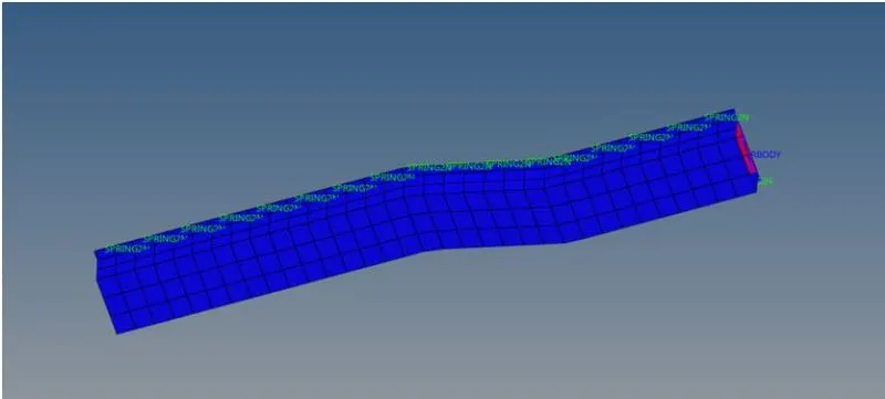
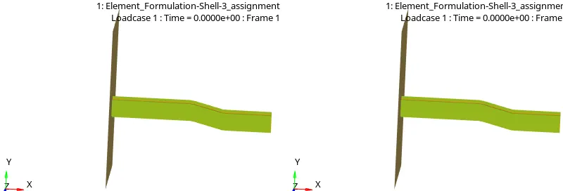
In this case the value for the shell property card, the values are kept what they are given i.e default. The analysis is ran without the changes. The process includes importing the given analysis file. The schematic of the component is shown below,
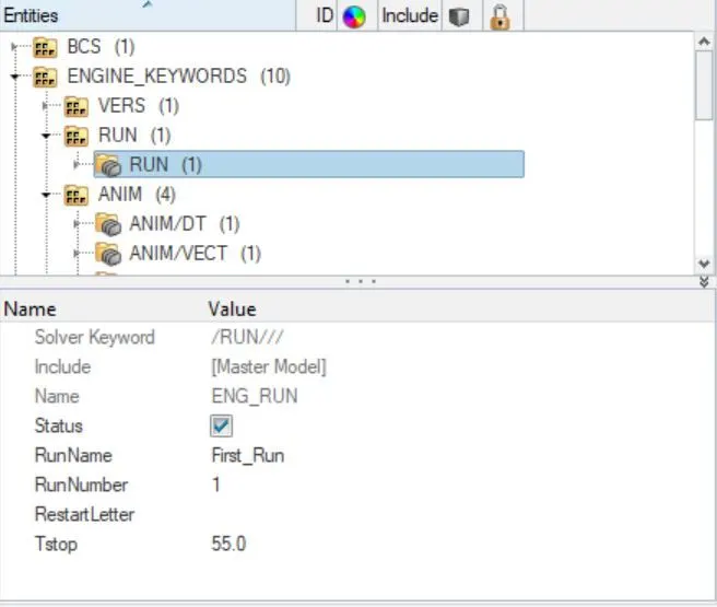
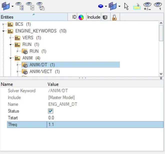
One of the objective is to run the simulation for 55ms. So in ENGINE RUN card the value is changed to 55ms. The another objective is to set the time interval of 25 to 60 animations over the entire simulation. The value is selected as 50 animation steps. So in ENGINE ANIM DT card the Tstart is set to 0 and Tfreq is set to 1.1
The default property card for shell elements is shown below,
The next step is to run the simulation. The RADIOSS option in Analysis is used. To perform the analysis faster 4 cores of the system are employed by entering -nt 4 as shown below, where nt stands for the number of threads and 4 is for 4 core CPU if 8 core CPU is available -nt 8 can be written. And click on Radioss which will start the run.
After successfull completion of the analysis it is now the post processing part. It can be seen that in the analysis folder total 51 files are printed with A001 to A051 as the first file of 0 time is with name A001.
The next check to perform is to see the energy error in the 0001.out file of the analysis. Below figure shows the energy error for this run at the end of the simulation.
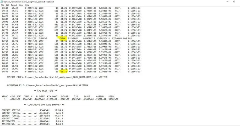
It can be seen that the energy error is almost -11.5%. The acceptable range for the energy is error from -15% to +5%. Basically it says that the energy is dissipated from the system. The main reason for this could be hourglass, i.e non physical modes of deformation. To check the energies the h3d file is opened in the hypergraph and the contours are observed in the hyperview.
Case 2: Recommended Values for the Shell Element Property Card
Following are the values for the shell element property card with all other settings similar to the case 1.
Ishell = 24
Ish3n = 2
Ismstr= 2
N = 5
Iplas = 1
Ithick = 1
Post Processing
i. Von Misses Contour
Following diagram shows the von misses contour for both the cases,
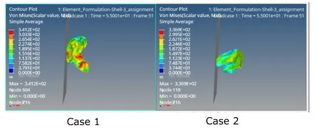
It can be seen that the stresses recorded in case 2 are lower than that of the case 1. To understand the reason for this it is important to look at the energy plot of both the simulations, Using the hyperplot the energies for both the simulations are plotted. Following figure gives the energy plots for both the simulations,
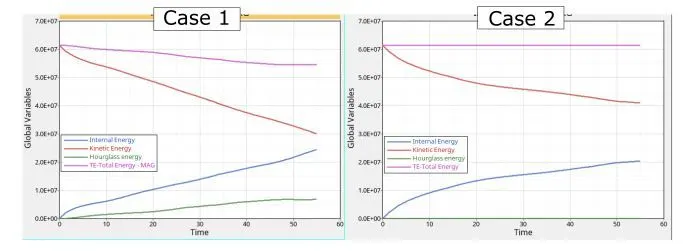
It is fundamental to know that energy can neither be created nor be destroyed but only it can be converted from one form to another. It can be seen that for Case 1 the Total Energy of system is falling over the course of simulation while the total energy for case 2 stays almost constant, this states that energy from system is lost for case 1 and i.e it is lost in the form of hourglass energy. This states that in case 1 the non physical deformation of element is occuring resulting into hourglass modes. As this energy is not accounted in the simulation. As the strain due to this is not recorded in the element, the stresses are not accurate. So the reason for wrong stresses is due to presence of the hourglass deformation. The reason for higher value of stress is due to a small amount of extra energy absorbed in process of the hourglass deformation of the elements (as it can be seen the internal energy for case 1 is higher than case 2). If the energy error percentage is seen, for Case 1 it is -11.3% while for Case 2 it is almost 0. Hence Case 2 gives accurate results.
ii. Forces on the Rigid Wall
Following is the plot for the Rigid wall forces for both the case,
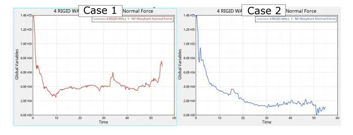
From the plot it can be seen that at the time of impact both the cases result same force. Eventually after the course of simulation the force decreases gradually for case 2 while in case 1 it increases. The most important reason is the contact area. For Case 1 the contact area is higher in the later part of the simulation whereas for the case 2 the area remains almost same.
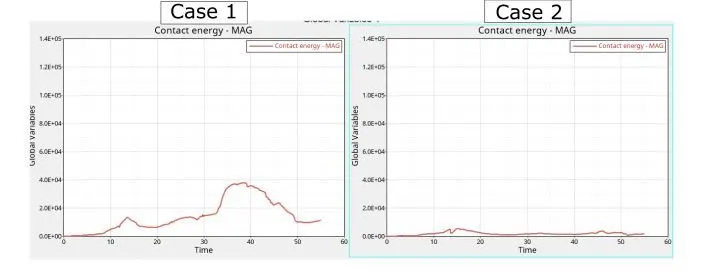
One interesting additional reason could also be possible that the case 1 element formulation is more stiffer than element in case 2. Investigation is needed to conclude this statement.
Conclusion:
Based on the results, it is clear that with the QEPH element formulation for shell element and the other recommended values for the property card of shell elements the results are accurate than default settings. The time required for case 2 (12.4s ) is higher than case 1(10.1s). But the accuracy is higher. Considering the cost and accuracy the recommended settings are best to use in practise.
In this assignment following outcomes were learned,
Understanding the Element Formulations.
Changing the Control Cards in the simulation and running the simulations.
Post processing using hyperview and hyperplot, i.e plotting the energy graphs and stress contours.