Assignment 3

Describing the difference of simulation result on the basis of shell element properties.

Introduction:

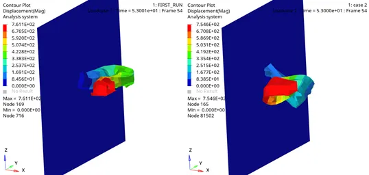
From the above picture, you might have found a difference in the deformation method. So, this paper is all about the difference of element properties and their significance in simulation to get accurate results. I will be talking about default shell element properties in RADIOSS and improved shell element properties. It is always good to perform simulations with high-grade shell properties however computing power imposes us to fall back and find optimal shell properties to balance cost and time and accuracy.

Internal Energy and hourglass energy is the best way to start to know the difference whereas it is subtle sometimes but mostly magnificent.

Model and Definitions:

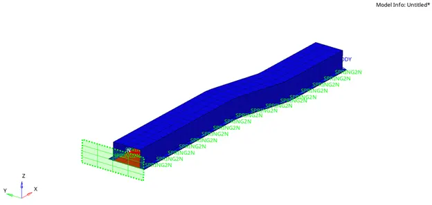
Understanding the model is inevitable. It is like INPUT. So, it's like you'll harvest what you sow. In about model, you can see a RIGID WALL (TRANSPARENT RECTANGULAR ELEMENT), QUAD4 SHELL ELEMENT, RBODY (Many nodes rbe2), SPOTWELD (SPRING2N ID ELEMNT).

Rigid wall: It is an infinite wall with infinite stiffness. No element or node can penetrate through this. No matter what.

Spot-weld:

RBODY: It is a special type of connection that transfers the same amount of force through all connected links. In RADIOSS, there are 3 types of RBODY i.e. making the body rigid, creating connection, to model non-modeled components.

These are the modeling component used for simulation. Note that no constraint is applied between the rigid wall and crush tube in this case and hence crush tube is not attached. It is just pushed against the rigid wall.

Boundary Conditions:

• This is the place where you give the command to the modeled component to do this and that. So, in this case, I want the crush tube to move with 6 mm/ms towards the rigid wall. I also don't want the crush tube to penetrate (without considering the effect of penetration) their own body while crushing. So to prevent self-penetration, a self-contact interface is required. That's it. Another is to make a strong bonding between the upper parts of the crush tube with the lower part as we don't want the lower part to detach while crushing (means consider both parts as a single part).

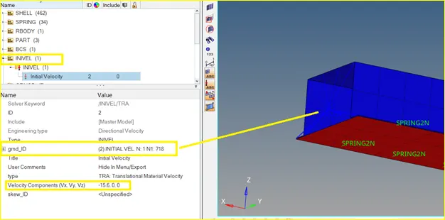
• To create, go to SOLVER DECK> RIGHT CLICK> CREATE> BOUNDARY CONDITIONS> INIVEL (same velocity for case 1 and case 2). Then after you can generate the initial velocity cad. Here as shown above the node selected for velocity is the master node of RBODY which transfer the same velocity to all node connected with the master node at every circumstance.
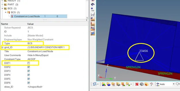
• Another boundary condition is to constrain the body to move in only one direction. This ensures that there is no deviation and pure orthogonal motion will be obtained.

• Type7 Interface:

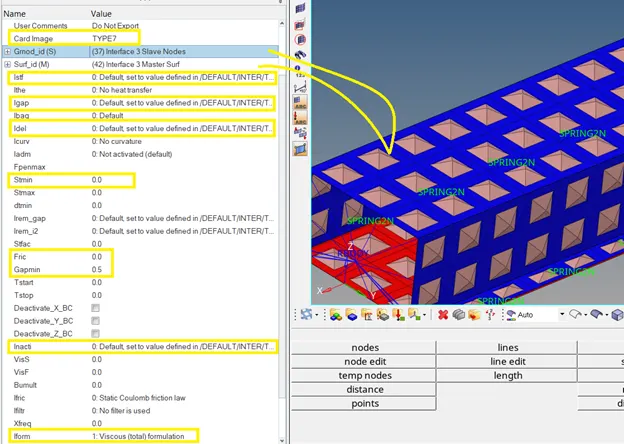
In this case, we are setting interface properties value to default (in this case Gapmin and Iform is changed trivially). Let's understand what happen if you leave all parameter to default one by one:

Istf: it will set the value to 1000 which means the stiffness of the contact interface will be computed from the master side only.

Igap: It will set the value to 1000 which means the gap is set to a constant which is inherited from Gapmin.

Idel: It will set the value to 1000 which means no deletion of nodes and shell.

Gapmin: It is the minimum gap required to activate the interface. It is essential in case of high-speed impact analysis to prevent penetration and failure of simulation (for the sake of proactive).

Inacti: It will set the value to 1000 which means no action is taken if there is initial penetration in the model (indifference).

Iform: It will set the value to 1 which means viscous formulation will be activated to calculate friction force between slave and master segment. (Preferred for explicit simulation).

• Type2 (Tied)Interface:
  • Between upper part and Spring2n:

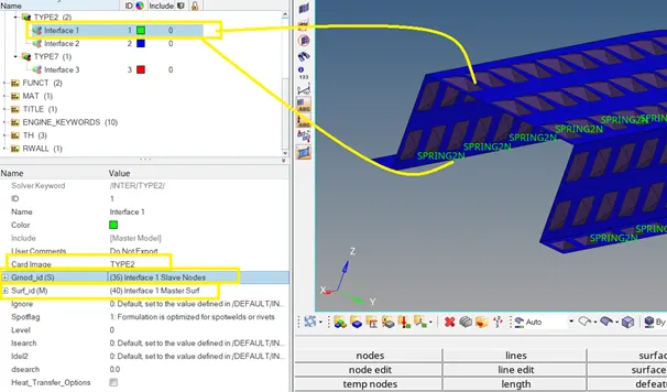
In order to create you need to select the set of nodes for slave and surface for the master. Then it creates a tied contact between them and nullifies the relative motion between those nodes.

Now, let's have 3 insight about type2 interface:

1. It can be used between shell, and shell and spring, and brick elements.
2. Using Spot flag=1, this is suitable for the spring element and no hourglass problem will arise.
3. Connection stiffness will be constant (Courtesy: Altair Hypermesh)

• Between lower surface and spring2n:

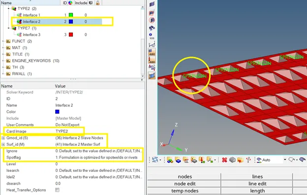
Now, let's talk about the last setup. Different shell properties which are different for both cases.

Shell properties:

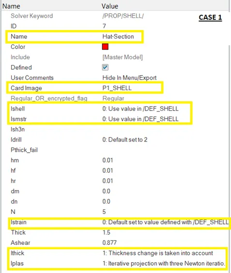
The shell properties for the case 1 is given below which is the default in this case except a number of integration point (N=5), Ithick and Iplas.

The shell properties for case 2 are given below which is an optimal value for simulation. However, the time taken for the simulation will increase. This will be huge in case of heavy simulation.

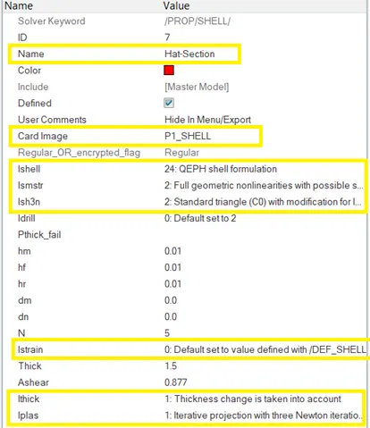
Differences in properties and their meanings:

Case/parameter	Ishell	Ismstr	Ish3n
Case 1	0: It is Q4 Belytschko which uses the perturbation method to control hourglass formation.	0: mean value is set to 2 by default which is full geometric non-linearity with possible small strain formulation.	<OFF>: It is used for trias and not used for calculation in this case.
Case 2	24: It is QEPH (An advanced element with one integration point) which uses the physical stabilization method to control hourglass formation.	2: It is the same as case 1.	2: it is a default triangle shell type that is used for large rotation. Note: no triangle elements are there in the model.

Results:

It is always good to start reviewing our results from ERROR %, hourglass energy, and mass error. So, we can decide whether the simulation results are acceptable or not. To check our results 0001.OUT file is shown below:

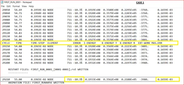
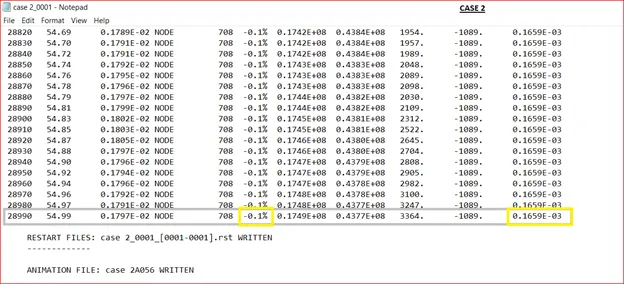
In both cases, you can see that energy error is between ±15percent which is an acceptable range. Here we can note the difference in using different shell properties. In case 1, the energy error is -10.3% where in case 2 the error is -0.1% only. This is due to the physical stabilization method used in controlling the hourglass formation. The addition of mass is also very less in both cases and the same. Hence, we proceed with our probation ahead to validate the result.

• Internal Energy and Hourglass:

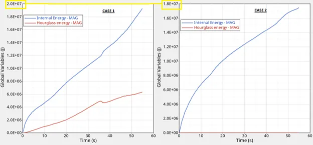
From here, it is obvious that the internal energy of the system is altered due to shell properties.

What is the role of the hourglass?

Hourglass is anomalous deformation that occurs due to bad mesh quality in reduced integration point shell.

How it affects internal energy?

From plot case 1, you can imply that the unnecessary deformation is adding energy to the internal energy of the system where this deformation is not supposed to exist in the simulation because this is not actual world deformation (never happened in reality).

From plot case 2, hourglass energy is totally zero means no unnecessary addition of energy in the system. Hence, this internal energy is more relevant to real-world deformation.

Let's do some mathematics:

From case 1, % error is -10.3:

Energy error becomes = 1.9E6

Actual energy becomes =1.9E7-1.9E6 = 1.7E7 (which is equal to the value in case 2)

• Displacements:

This is an easy way of interpreting the results. It is visible. One can use their intuition to contemplate whether the deformation is sensible or not. So, let's check it for both cases and compare.

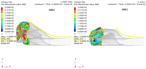
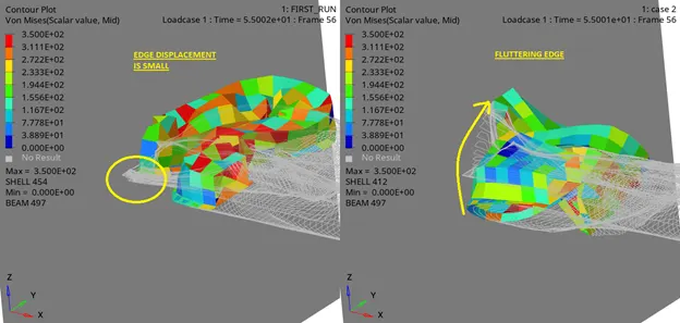
If you remember the modeling, boundary conditions, and shell properties definition then you might possibly know that only shell properties are different. Therefore, we can say that the change in deformation pattern is due to the shell properties definition. In case 1, the deformation is excessively high in Y-direction. In case 2, you can see the fluttering of the corner and it is because the deformation is in control which is not in case 1.

Rigid wall force:

The force acting on the rigid wall will give us insight into how the body is interacting with the rigid wall and also give us an idea about the deformation with time. The larger the contact of the body the larger the force magnitude. The picture given below is depicting the varying force acting on the rigid wall with time and contact.

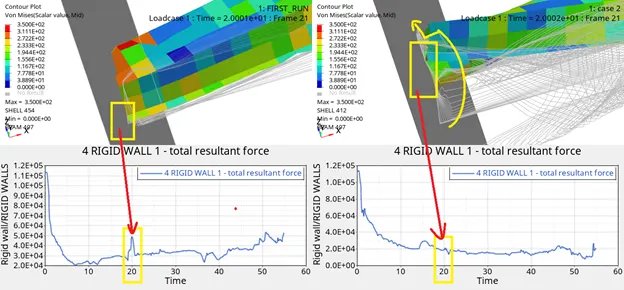
So, for comparison purposes take the time around the 20 second wherein you can see the hike in force in case 1 due to increasing contact around 20 second but that is not the case in case 2. In case 2 the force keeps decreasing around 20 seconds. This is a great observation if you're performing a time-domain analysis.

Initially crush tube was more straight and contact was 100% hence force on the rigid wall was high but kept decreasing as time passes. Because the tube started to deform and normal force acting on the rigid wall also started to dissect in other than normal to rigid pole directions and tube contact is decreased.

Contact Energy:

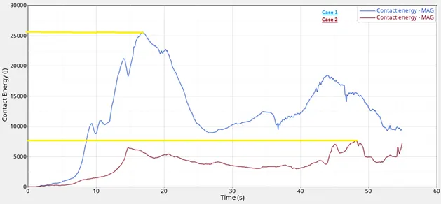
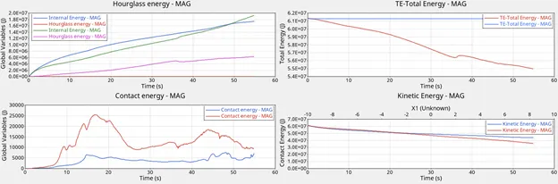
Contact energy between 0-5percent is acceptable. In this scenario, the maximum contact energy in case 1 is around 25500 (0.04% of total energy) between 10- 20 seconds whereas the maximum contact energy in case 2 is around 7500 (0.012% of total energy) between 40- 50 seconds. Indeed, the simulation result is acceptable for both cases in terms of contact energy.

Total Energy:

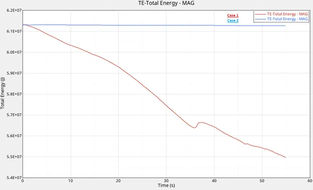
Initially, the system is under zero energy state until and unless the external excitation force is applied. The term "total energy" is the energy of the system. In this case, we subjected initial velocity on the body (crush tube) to mean kinetic energy. Note that at time t=0,

Kinetic energy = total energy of the system

As time passes, deformation continues and kinetic energy will be disseminated in many other forms meantime the total energy of the system must remain constant i.e. equal to the initial kinetic energy, according to the law of conservation of energy.

In case 1, the above statement does not seem to be obeyed. The total energy of the system is decreasing linearly which is due to hourglass energy and contact energy.

In case 2, the above statement is obeyed almost nearly. The magnitude of the total energy of the system is constant throughout with little variations.

Overall Results:

Learning Outcomes:

• The difference of using the various shell properties during simulation
• Way of analyzing the result from energy error and mass error.
• Interpreting the result in terms of internal energy, hourglass energy, contact energy, kinetic and total energy
• Significance of visualizing the displacement to check innateness

Conclusion:

Shell properties have a great impact on the result of the simulation so it is recommended to select optimal properties for the shell while taking computational time into consideration.