CRASH BEAM SIMULATION IN RADIOSS

AIM :

• To interpret the force and energy results by comparing the results of crash beam simulation in radioss which are carried out with default input values and simulation with improved shell element properties.

OPERATIONS INCLUDED :

1.Using the crash beam file from the previous assignment, change the run time to 55 ms.

2. Change the number of animation steps during simulation to a minimum of 25 and maximum of 60.

3. Run the base simulation without any modification to element properties.

4. At the end of the simulation, do the energy error and mass error checks and determine whether results would be acceptable.

5. If acceptable, Plot rigid wall forces, internal energy, hourglass energy, contact energy, total energy of the simulations.

6. Change all the shell elements properties to recommended properties, save this as separate, rad files and run the simulation.

RECOMMENDED PROPERTIES :

Parameters		Comment
Ishell =24		QEPH 4 nodes shells are best combination of cost and accuracy.
Ismstr=2		Full geometric nonlinearities (default)with possible small strain formulation activation in RADIOSS Engine.
Ish3n=2		Standard 3 noded shell (C0)with modification for large rotation(default)
N=5		Number of integration points set to 5 for accuracy bending.
Ithick=1		Thickness change is taken into account for accuracy.
Iplas=1		Iterative plasticity for good accuracy

THEORY :

Hourglass modes are nonphysical, zero-energy modes of deformation that produce zero strain and no stress. Hourglass modes occur only in under-intetgrated (single integration point) solid, shell, and thick shell elements. They produce no stress. Under-integrated elements have just one integration point. This under/reduced-integration result in hourglass modes.

There are two methods used to control formation of hourglassing.

• Perturbation (Q4)
• Physical stabilization (QEPH).

1) Perturbation/Viscous method:

This method is used by the solver when the hourglass deformation mode is detected with the relative velocity of the nodes. A damping force is applied to oppose this velocity. This results in addtition of stiffness to the elements and the deformation is then stabilized. This force introduces an artificial energy.

This method is used to inhibit addition hourglass deformation from the point hourglassing is detected. It does not help the system recover from previously accumulated HG deformation.

This method is used for high velocity/high strain rate problems.

2) Physical stabilization/Stiffness method (QEPH):

For the hourglass stabilization, this method works on a material level. Hourglass loading depends on natural tangent modulus and the stiffness is added to the material.

QEPH is also able to reduce total accumulated hourglassing deformation and is preferred for low strain rate problems. It is also the best method that is both inexpensive and accurate.

For our second case, QEPH is preferred.

PROCEDURE :

CASE 1 : SIMULATION WITHOUT MODIFICATION TO ELEMENT PROPERTIES.

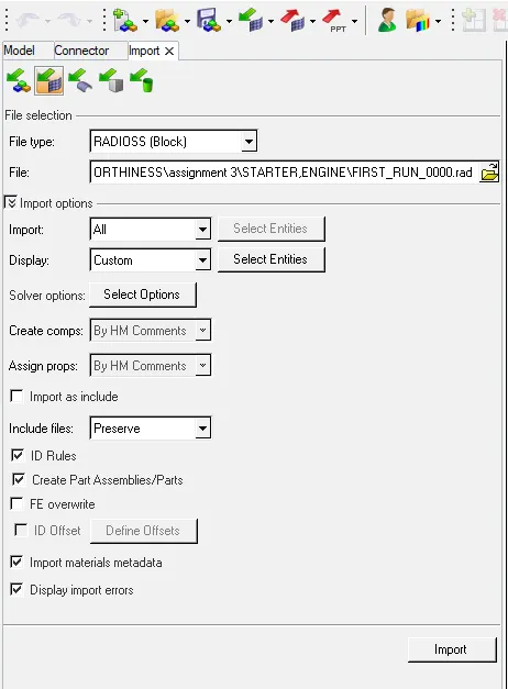
open hypermesh with radioss profile and then using the import solver deck button( )available in menu bar and then we will hit the suitable file type as radioss(block) and choose the starter file to import. basically starter file have all the input details about the model setup like components,mesh nodes/elements information ,material laws,contact details,boundary conditions etc.,

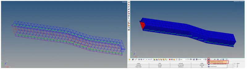
after importing the model might be visible to us in wireframe mode which we can turn it into shaded mode by selecting "shaded elements and mesh lines" button available under graphic area as shown below.

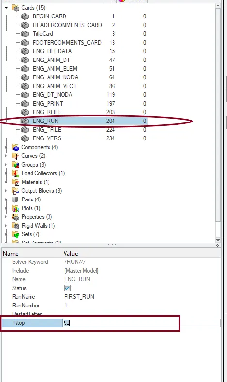
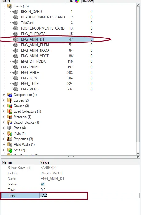
after importing the model we will calculate and edit the Tfreq to such a value that during simulation it will gives output of animation step files that lies between 25 and 60.here we took 36 as a average value that lies between 25 and 60.so after substitutingvalue 36 in Tfreq formulae which is ` Tfreq = Δt/no.of animation step files `where Δt is Tstop value which we should give 55.ie., the simulation runs for 55ms . so therefore Tfreq=55/36 which gives result of 1.52.now we will edit that 1.52 value in Tfreq property tab that available under ENG_ANIM_DT card. and then Tstop 55 value to ENGINE_RUN card as shown below.

after that we proceeded for simulation in radioss without changing any material properties.to perform simulation we go to Analysis-radioss in menu as shown below

right after selecting radioss we will be redirected to the tab that let us choose the path to save the input file while simulation happens which contains starter file.engine file animation file,output file etc that have all the data of simulation.here in this case we created a separate new folder named "before" so that we wont be confused between the files that we get after applying improved shell element properties.right after choosing the path for input file we wrote -nt 4 command under options tab that helps the software to run the simulation smoothly.then finally we click on "radioss" button to run the simulation.

Right after clicking radioss we will see a popup window that running all the commands in engine input file as shown below.

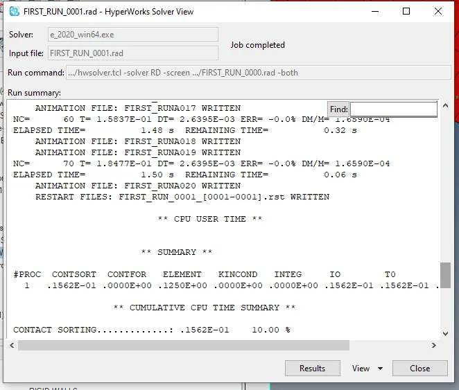
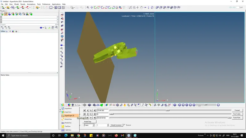
we can see how many animation files are written and how much time it took to run the simulation and all other extra information in that hypersolve window that popped up.to view the animation and graphical representation of the simulation we can just click on the results tab that present at the bottom of the window.Now, as all the analysis is done and to see kinds of results, we need to switch the view type to different type like from HyperMesh to HyperView or HyperGraph 2D. But before that we need to understand few things from the data, we got in the designated folder during solving of model.

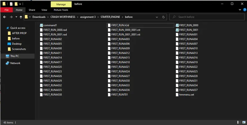
If we see that folder, we will find several files of different extensions like .h3d, T01, 001.out etc. So, in radioss h3d file is the file for animation which is actually a combined file of all A001-A038 file formed in folder and the number of A file in folder depends on the frequency we set in engine file. T01 file is the file used for plotting different kinds of plots, And 0001.out file will contains several information out of which we have parameters of concerns like energy error and mass error checks.

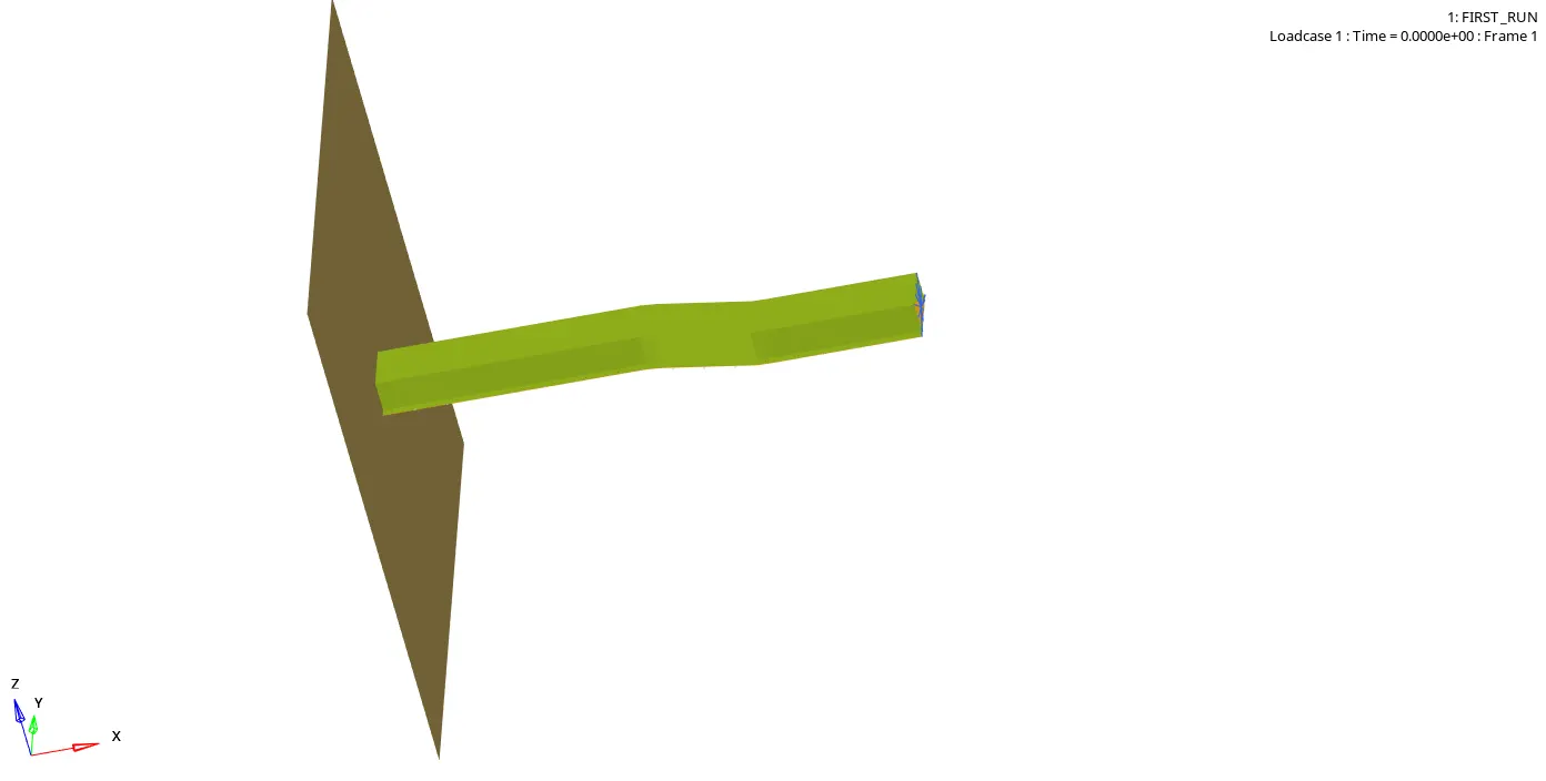
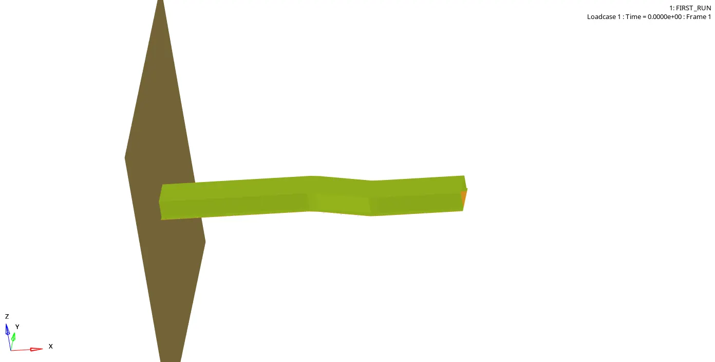
below is the gif file that shows us how deformation occurs in an animation file that runs with 38 frames.there are 38 animation files are created in the new folder we created,which is result for the input we gave i.e., Tfreq as 1.52.

here we plot the graph for the simulation that happened above. the graph plot include how the energies are varying with respect to time ie., internal,contact,total energy and hourglass energy.the graphs are plotted by opening the Hyperview 2D- open T01 file.

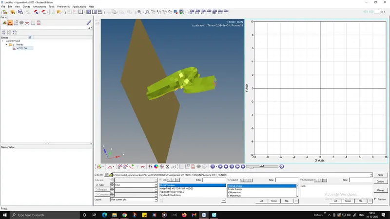
From the above computations energy plots like hourglass energy, contact energy, internal energy, total energy are plotted and forces like Rigidwall forces/Rwall force are also plotted which is shown below.

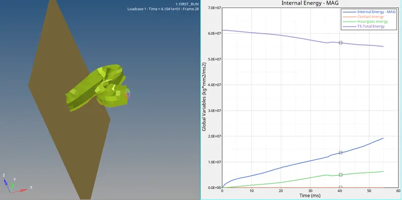
If we check the plotted graphs, hourglass energy keeps on increasing with respect to time which states that the hourglass error is taking place which may be the cause for other types of energy errors like internal,contact and total energy.

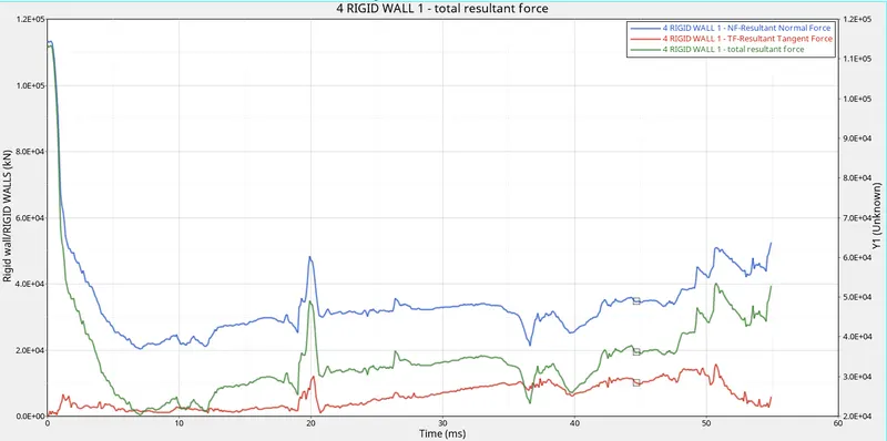
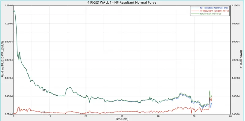
Due to contact and friction between the crash beam and the rigidwall. Normal force is applied onto the rigid wall during simulation. This force keeps on decreasing as the simulation progress and simultaneously, much of normal forces are converted into frictional forces. These forces are plotted along with the resultant forces.

we need to check values of energy error and mass error from 0001.out file created in designated folder whether they are acceptable or not.It can be done by opening engine out file in notepad.

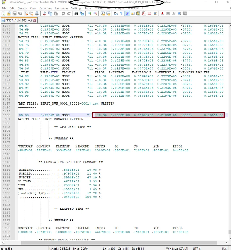
So, for the simulation type without property change we observed that energy error is fluctuating from 0.0% - (-10.3%) and mass error was 0.1659E-03 for every time step which depends on frequency, we set in engine file.These are acceptable energy errors since, the energy error value range is between -15% to -5% . The negative energy errors can be attributed to hourglass energy modes being generated in the simulation file.

CASE 2 : SIMULATION CONSIDERING THE IMPROVED SHELL ELEMENT PROPERTIES

After importing new input file of the same rail component and repeating the same steps we followed earlier for Tstop and Tfreq value .we will change the properties as listed in the challenge.

Parameters		Comment
Ishell =24		QEPH 4 nodes shells are best combination of cost and accuracy.
Ismstr=2		Full geometric nonlinearities (default)with possible small strain formulation activation in RADIOSS Engine.
Ish3n=2		Standard 3 noded shell (C0)with modification for large rotation(default)
N=5		Number of integration points set to 5 for accuracy bending.
Ithick=1		Thickness change is taken into account for accuracy.

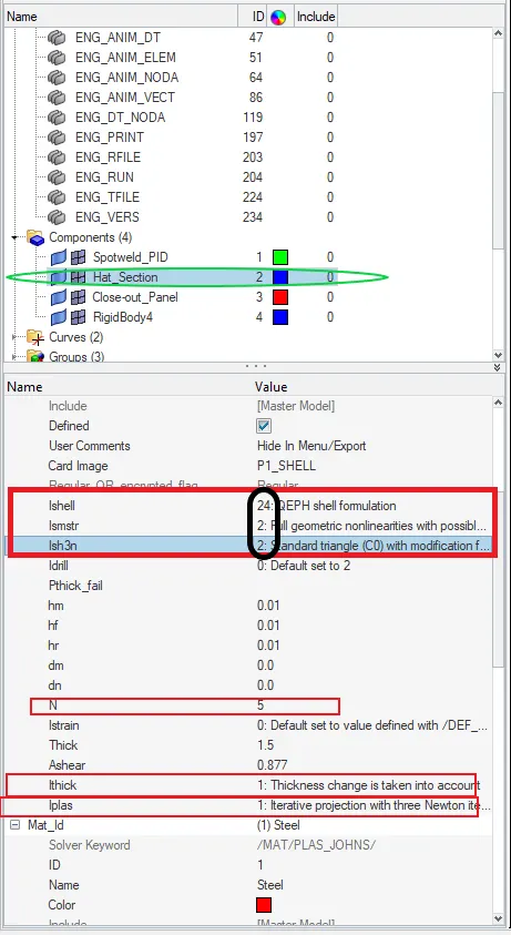
after changing the property values we will run the simulation in radioss platform.the deformation is demonstrated in gif format below.we can observe that the deformation varies comparing with the previous simulation ie., the body is getting deformed in a proper way since we considered the property values which gives us somewhat better results after resolving the hourglass errors that happened before.

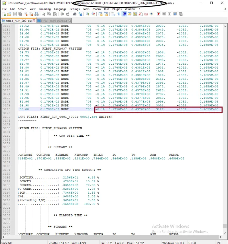
It can also be observed that due to change in property parameters the energy error is improved from case 1 -10.3% to case 2 -0.1% and the mass error stays the same ie., 0.1659e-03.

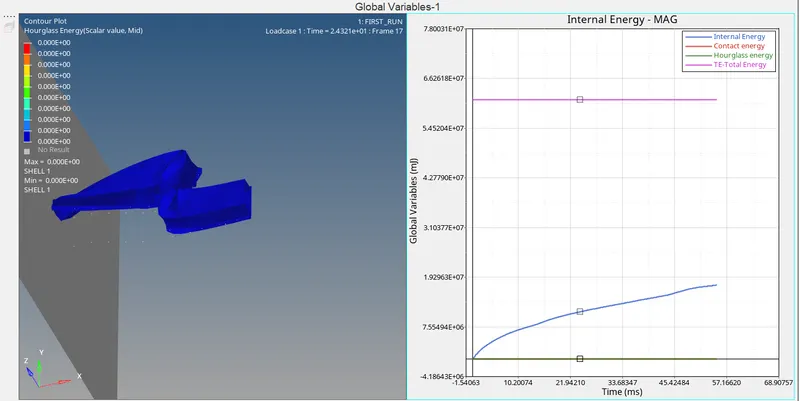
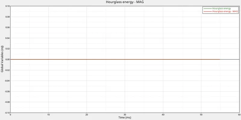
if we plot the graph again for all the energies we want to see .we observe that Hourglass energy becomes zero because of QEPH shell formulation. Internal Energy increases gradually as the time increases.Total Energy Remain constant and Contact Energy Remain Constant and equal to zero.

From the rigid wall forces obtained in both the cases, it can be observed that for case 1 as the simulation progress the normal force decreases and there is little variation as the property parameters are kept default but in case 2 as the elements property parameters are changed it can be observed that there is a huge spike in normal and tangent force because of the improvement in the shell element formulation.

RESULT :

• Due to change in property parameters the energy error is improved from -10.3% to -0.1% and the mass error stays the same ie., 0.1659e-03.
• By the end of the simulation we can conclude that the Hourglass effect almost reduced to zero because of QPEH shell formulation.