Analytical study of the real time Drive cycle using Driver Glider Model and modeling of GM EV1 car for Wide Open Throttle calculation.
Aim: Analytical study of the real time Drive cycle using Driver Glider Model and modeling of GM EV1 car for Wide Open Throttle calculation.
Formulae:
01.
Motor Torque (Tm):
`Tm = frac {Fte times r} {G}`
Fte = Total Tractive Effort.
r = Tire radius in mm.
G = Gear ratio.
02.
Wheel Torque or Axle Torque (Tw):
`Tw = Fte times r`
Fte = Total Tractive Effort in N.
r = Tire radius in mm.
03.
Angular speed of the motor shaft `(omega)`:
`omega =frac{v}{r} times G`
v = Linear velocity of the vehicle m/s
r = Radius of the tire in mm.
G = Gear ratio.
04.
Rolling Resistance Force (Frr):
`Frr = murr*m*g`
μrr = Coefficient of rolling resistance.
m = Total mass of a vehicle in kgs.
g = Gravitational acceleration m/s^2.
05.
Aerodynamic Darg Force (Fad):
`Fad = frac{1}{2}*rho*A*Cd*v^2`
⍴ = Density of air kg/m^3.
A = Cross sectional area of vehicle front mm^2.
Cd = Coefficient of drag.
v = Velocity of vehicle in m/s.
06.
Hill Climbing Force (Fhc):
`Fhc = m*g*sinpsi`
m = Total mass of the vehicle in kgs.
g = Gravitational acceleration in m/s^2.
Ψ = Angle of climb in radians.
07.
Linear Acceleration Force (Fla):
`Fla = m*a`
m = mass of the vehicle in kgs.
a = Linear acceleration of the vehicle in m/s^2.
08.
Angular Acceleration Force (Faw):
`Faw = Ir*frac{G^2}{r^2}*frac{a}{etag}`
I = Moment of Inertia of circular section.
G = Gear ratio.
r = Radius of the tire in mm.
a = Linear acceleration of the vehicle in m/s^2.
ηg = Efficiency of the gear system.
09.
Total Tractive Effort (Fte):
`Fte = Frr+Fad+Fhc+Fla+Faw`
Frr = Rolling Resistance Force in N.
Fad = Aerodynamic Drag Force in N.
Fhc = Hill Climbing Force in N.
Fla = Linear Acceleration Force in N.
Fwa = Angular Acceleration Force in N.
10.
Vehicle Propulsion Power (Pte):
`Pte = Fte*v`
Fte = total Tractive Effort in N.
v = Velocity in m/s.
Objectives:
To study the concept of power requirements of the vehicle under different loading conditions while hill climbing.To study concept of gradeability and design the flyover for a vehicle (truck) climbing a summit of height 5.5 meters.To study and prepare your own drive cycle.To study and modeling of the WOT (Wide Open Throttle) response of GM EV1 car.
Introduction:
A driving cycle is a series of data points representing the speed of a vehicle versus time.
Driving cycles are produced by different countries and organizations to assess the performance of vehicles in various ways, as for instance fuel consumption, electric vehicle autonomy and polluting emissions.
Fuel consumption and emission tests are performed on chassis dynamometers.
Tail pipe emissions are collected and measured to indicate the performance of the vehicle.
Another use for driving cycles is in vehicle simulations. More specifically, they are used in propulsion system simulations to predict performance of internal combustion engines, transmissions, electric drive systems, batteries, fuel cell systems, and similar components.
Driving cycle design is the core technology for these standard cycles. Optimization and Markov chains are employed to design a driving cycle. Drive cycle recognition is applying to Hybrid Electric Vehicle.
The "Drive-cycle" basically is the representative of the road.
Drive cycles are used to reduce the expense of on road tests, time of test and fatigue of the test engineer.
The whole idea is to bring the road to the test lab (a chassis dynamo-meter) or to the computer simulation.
Two kinds of drive cycle can be made.
One is DISTANCE DEPENDENT (SPEED versus DISTANCE versus ALTITUDE) and the other one is TIME DEPENDENT (SPEED VS TIME VS GEAR SHIFT).
The DISTANCE DEPENDENT is the actual replica of the test road whereas TIME DEPENDENT is the compressed version of the actual time taken to conduct the test on road.
Examples of TIME DEPENDENT drive cycles are European NEDC cycle, FTP-75.
TIME DEPENDENT drive cycles are used specifically for chassis dynamo meter testing because in a short time the results can be availed and repeated tests can be done easily.
Problem Statement:
01. What is the ratio of hill-climbing power required by fully loaded tata ultra truck to the half-loaded one?
02. A flyover is planned to be constructed on a national highway. Keeping in mind about the gradeability for trucks, how much can be the minimum length of the flyover, considering the minimum height at the summit should be 5.5 meters? State your assumptions.
03. Prepare a new drive cycle excel file for the model and also include a hill-climbing angle to it. Revise the model file “Driver_Glider.slx” and comment on the results.
04. Model the WOT (Wide Open Throttle) response of GM EV1 car. Compare it with the official figures of the performance of a real vehicle. Prepare a table showing variation in acceleration time with a 5% change in vehicle parameters.
Solution:
01.
To study the concept of power requirements of the vehicle under different loading conditions while hill climbing.
Assuming following data for given conditions:

Velocity of the vehicle (v): 30 kmph.

Angle of hill climbing (Ψ): 20֯.

Acceleration due to gravity (g): 9.81 m/s.

Kerb weight of the vehicle (Tata Ultra Truck): 7500 Kgs.

Partially loading capacity : 5.1 tons.

Fully loading capacity : 10.2 tons.
A. For Partially loaded vehicle:

   Velocity (v): 30 kmph

               = 8.33 m/s

   Angle of hill climb (Ψ): 20

               = 0.3488 radians.

   Partially loaded capacity: 5.1 tons

               = 5100 Kgs.

   Total mass of a vehicle = 7500 + 5100

               = 12600 Kgs

   Force required by the vehicle to overcome the hill climbing resistance (Fhc1) = mgsinΨ

                                                                                 = 12600 * 9.81 * sin(0.3488)

                                                                                 = 752.47 N

   Power required for the vehicle during hill climbing (Phc1): Fhc1 * v

                                                             = 752.47 * 8.33

                                                             = 6268.07 W

                                                             = 6.3 KW
B. For Fully loaded vehicle:
Velocity (v): 30 kmph
= 8.33 m/s
Angle of hill climb (Ψ): 20
= 0.3488 radians.
Partially loaded capacity: 10.2 tons
= 10200 Kgs.
Total mass of a vehicle = 7500 + 10200
= 17700 Kgs
Force required by the vehicle to overcome the hill climbing resistance (Fhc2) = mgsinΨ
= 17700 * 9.81 * sin(0.3488)
= 1057.04 N
Power required for the vehicle during hill climbing (Phc1): Fhc1 * v
= 1057.04 * 8.33
= 8805.18 W
= 8.8 KW
Therefore the ratio of Phc2:Phc1 = 8.8:6.3
Phc2/Phc1 = 1.4 02.
To study concept of gradeability and design the flyover for a vehicle (truck) climbing a summit of height 5.5 meters.
    Assuming following data for given conditions:


    Gradeability of truck = 20 %

    Height of summit = 5.5 meters

    But,

      Gradeability = frac{RISE}{RUN}*100`

    Therefore,

      `20 = frac{5.5}{RUN}*100`

    Therefore,

      RUN = 27.5 meters.

      That means for climbing 5.5 meters of vertical distance (RISE) vehicle will have to travel 27.5 meters of      horizontal distance (RUN).

      This horizontal distance is nothing but the length of the flyover for the summit of 5.5 meters.

      Therefore length of flyover (Lf) = 27.5 meters.
03.
To study and prepare your own drive cycle.
We konw that A driving cycle is a series of data points representing the speed of a vehicle versus time. Driving cycles are produced by different organizations to assess the performance of vehicles in various ways, as for instance fuel consumption, electric vehicle autonomy and polluting emissions.
For the study here we prepared our own drive cycle in the excel sheet which can be asessed by using following link.
To study the drive cycle we used the Driver Glider model of the simulink. The main purpose of our study isto examine how our vehicle is responding to our instructions as per drive cycle and we can do it by plotting plot for drive cycle. Driver Glider Model considers the angle of gradeability and calculates the forces acting on the vehicle accordingly; while vehicle is running as per our drive cycle. Therefore the forces produced by the vehicle should be such that the actual speed must match the reference speed (Speed mentioned in the drive cycle). Here for the study we took the angle of gradeability as 2.
Following steps were followed to study the drive cycle in Driver Glider Model:
A. Open Matlab and goto "HOME" and now click on "Import Data".
B. Import the Excel file of the drive cycle by clicking on "Open".
C. Select the "Numeric Matrix" from the "Import" tab opened.
D. Now click on "Import Selection".
E. Minimize the "Import" tab.
F. Goto "Current folder" and open the folder name "vehicle-modeling-master".
G. Now open the folder named as "VehicleModeling4p0".
H. Right click on the folder "VehicleModeling4p0" and create the path for the selected folders and subfolders.
I. Now open the folder named as "Simulink".
J. Now double click on "Driver_Glider_Library".
K. Click on the Lock symbol from the "Driver_Glider_Library" tab to unlok the model and minimize the tab.
L. Now open the folder named as "Glider" and double click on "Driver_Glider.xls".
M. Now simulink will open the Driver-Glider model. Now double click anywhere in the model in blankspace and type "from workspace".
N. And select the "From workspace" and rename the element also click the element once and press enter to open it.
O. Now copy the driving cycle from "workspace" and paste it in "data" from the element tab.
P. Click on "Apply" and then on "OK".
Q. Now delete the "US06" element and conect the recently made element of drive cycle.
R. Now double click in the blankspace and call for "Scope" and connect it to model instead of "Results".
S. Select the "Stop Time" as per our drive cycle and click on the "Run" to get the plot.
T. Now double click on the "Glider" and enter the value gradeability angle (6) select "Apply and "OK".
U. Run the model again to get the plot.
Following link gives the file for the study of Driver Glider Model:
Driver Glider Model for the study.
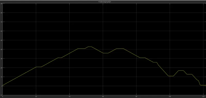
Figure01: Time Vs. Velocity plot for the drive cycle.
Figure01 shows the graph of time Vs. Velocity for a selected drive cycle. From the figure it can be concluded that the model approximately matches the reference inputs (Drive Cycle) with the actual outputs.
04.
To study and modeling of the WOT (Wide Open Throttle) response of GM EV1 car.
Here we will study the modeling of Wide Open Throttle (WOT) for GM EV1. In this we will change (Increasing by 5%) the all the given parameters of the GM EV1 and model the WOT and compare with the official figures.
In case of automobile, WOT is when the accelerator is fully pressed, referred as "flooring it".
In EVs WOT is referred to initial acceleration or time taken by the vehicle to reach the maximum velocity.
Maximum velocity in WOT condition can be obtained by electric motor characteristic of electric vehicle.
Modelling for WOT:
Following excel file shows data available for the comparision and study for WOT of GM EV:
Comparision of the GM EV1 Vehicle features.
Governing Equations for the WOT:

For traction force

`Fte = μrrmg + 0.625CdV^2 + ma + I frac{G^2}{ηgr^2}a`

                                                                        ...equation(1)

we know that,
Fte = T*v

But
v = G/r

Therefore'

`frac{G}{r}T= μrrmg + 0.625CdV^2 + (m + I frac{G^2}{ηgr^2})*frac{dv}{dt}`

                                                                        ...equation(2)


For ω < ωc in the initial acceleration we consider T = Tmax.


`frac{G}{r}*Tmax= μrrmg + 0.625CdV^2 + (m + I frac{G^2}{ηgr^2})*frac{dv}{dt}`

                                                                        ...equation(3)


where,

dv/dt = Acceleration in m/s^2.

g = Acceleration due to gravity.

I = Moment of Inertia.
For
velocity less than critical velocity.
we assume,
T = Tmax
And for velocity greater than critical velocity,
We know that,
Power = Torque * Angular velocity
P = T*ω
...equation(A)
But ω = v/r
...equation(i)
Substituting (i) in (A)
P = T*(v/r)
Therefore
T = P/(v/r)
Considering Gear ratio
we get,
T = P/G(v/r)
substituting corresponding values we get,
T 102000*0.3/11*v
T = 2757/v
A.

For given values of features of vehicle:

Case (i): Velocity is less than critical velocity (ω < ωc):

    Considering T = Tmax

    Now substituting all the correponding values into equation(3),

    Considering the efficiency of the coupling between motor and axle as 95%,

    We get,

    0.95*37*140 = 0.0048*1540*9.81 + 0.625*1.8*0.19*v^2 + 1560*dv/dt

    4921 = 72.51 + 0.213*v^2 + 1560*dv/dt

    4848.49 = 0.213*v^2 + 1560*dv/dt

    3.11 = 0.000137*v^2 + dv/dt

    dv/dt = 3.11 - 0.000137*v^2

                                              ...equation(4)

    Rewriting equation(4) in finite form

    Vn+1 = Vn + dt (3.11 - 0.000137*Vn^2)

                                              ...equation(4)


Case (ii): Velocity is greater than critical velocity (ω > ωc):

   Considering T = 2757/v

    Now substituting all the correponding values into equation(3),

    Considering the efficiency of the coupling between motor and axle as 95%,

    We get,

    0.95*37*2757/v = 72.4 + 0.214*v^2 + 1560*dv/dt

    dv/dt = 62.1/v - 0.046 - 0.000137*v^2

                                                             ...equation(5)

    Rewriting equation(5) in finite form

    Vn+1 =  Vn + dt (62.1/Vn - 0.046 - 0.000137*Vn^2)

                                                             ...equation(5)
B.
For 5% increased values of features of vehicle:
Case (i): Velocity is less than critical velocity (ω < ωc):
Considering T = Tmax
Now substituting all the correponding values into equation(3),
Considering the efficiency of the coupling between motor and axle as 99%,
We get,
0.99*37*147 = 0.0050*1638*9.81 + 0.625*0.89*0.1995*v^2 + 1638*dv/dt
5385 = 80.34 + 0.111*v^2 + 1638*dv/dt
5305 = 0.111*v^2 + 1638*dv/dt
3.24 = 6.78*v^2 + dv/dt
dv/dt = 3.24 - 0.0000678*v^2
...equation(4)
Rewriting equation(4) in finite form
Vn+1 = Vn + dt (3.24 - 0.000068*Vn^2)
...equation(4)
Case (ii): Velocity is greater than critical velocity (ω > ωc):
Considering T = 2980/v
Now substituting all the correponding values into equation(3),
Considering the efficiency of the coupling between motor and axle as 99%,
We get,
0.99*37*2980/v = 0.0050*1638*9.81 + 0.625*089*0.1995*v^2 + 1638*dv/dt
dv/dt = 66.64/v - 0.05 - 0.0000678*v^2
...equation(5)
Rewriting equation(5) in finite form
Vn+1 = Vn + dt (66.64/Vn - 0.05 - 0.0000678*Vn^2)
...equation(5)Following excel sheet shows the variation in the Acceleration time (Ta) with 5% change in vehicle parameters.
Variation in acceleration time (Ta) with 5% change in vehicle parameters.
Following image shows the graph for the WOT response when velocity is less than a critical velocity.
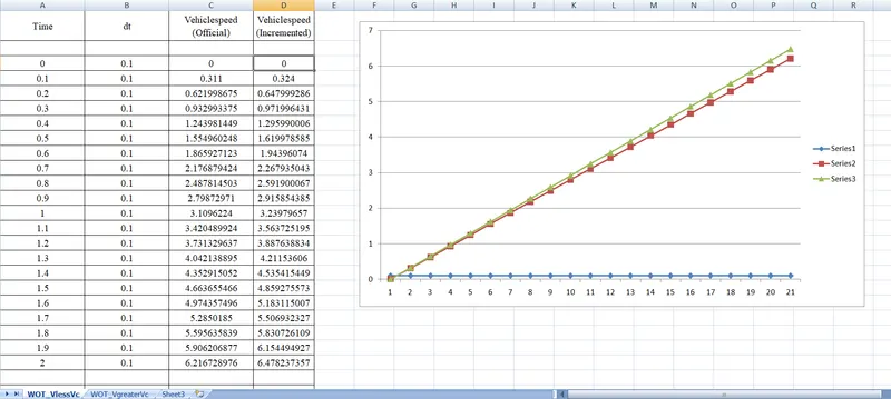
From the graph it can be observed that, The speed achieved by the vehicle in corresponding time while the parameters of the vehicle are increased by 5% is greater than the speed achieved by the vehicle in corresponding time while the official parameters of the vehicle are under consideration.
In other words we can say that the acceleration time decreases (Maximum speed is achieved within minimum time) while the parameters of the vehicle are increased by 5% as compared to the acceleration time achieved while the official parameters of the vehicle are under consideration.
Results:
From the study it can be concluded that Acceleration time required by the vehicle while the velocity is less than crical velocity while operating on official parameters is greater than acceleration time required by the vehicle while operating on the incremented parameters.