Study of Curve fitting for the best fit of the given set of data in Matlab.

Aim: To study the Curve fitting for the best fit of the given set of data in Matlab.

Objectives:

The study of curve fitting is done to understand the concept of the curve fitting and learn the programming for curve fitting to choose the best fit for the given set of data in matlab.

1. Introduction:

We often took a number of data points, obtained by sampling or experimentation, which represent the values of a function for a limited number of values of the independent variable.

              Curve fitting is the process of constructing a curve or mathematical function that has the best fit to a series of data points possibly subject to constraints. Curve fitting can involve either interpolation or smoothing in which a ‘smooth’ function is constructed that approximately fits the data.   

               In the mathematical field of numerical analysis, interpolation is the type of estimation, a method of constructing new data points within a range of a discrete set of known data points. It is often required to interpolate, i. e., estimate the values of that function for intermediate value of the independent variable.

               Fitted curves can be used as an aid for data visualization, to infer the values of a function where no data are available and to summarize the relationship among two or more variables. Extrapolation refers to the use of the fitted curve beyond the range of observed data. Thus it is subjected to a degree of uncertainty since it may reflect the method used to construct the curve as much as it reflects the observed data. 

1. Problem Statement:

                 Write code to fit a linear and cubic polynomial for the Cp data. 

                 Plot the linear and cubic fit curves along with the raw data points. 

                 Write a code to show split-wise method.

                 Explain the parameters used to measure the fitness characteristics for both the curves.

Program-01:
Code for linear polynomial using the Cp data:
01.	 % Programming the Curve fitting of Linear polynomial for a given data.
02.	
03.	clear all
04.	close all
05.	clc
06.	
07.	% Preparing data
08.	Cp_data = load('data');
09.	temp = Cp_data(:,1);
10.	Cp = Cp_data(:,2);
11.	
12.	% Curve Fit for linear equation.
13.	% Cp = ax + b
14.	Coeff = polyfit(temp,Cp,1);
15.	Predicted_Cp = polyval(Coeff,temp);
16.	
17.	% Plotting
18.	plot(temp,Cp,'linewidth',3,'color','g');
19.	% Compare my curve fit
20.	hold on
21.	plot(temp,Predicted_Cp,'linewidth',3,'color','r')
22.	
23.	xlabel('Temperature [K]');
24.	ylabel('Specific heat [KJ/Kmole-K]');
25.	legend('Original Data','Curve Fit');

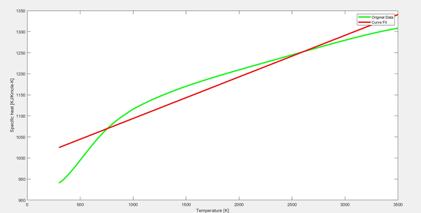
Figure01: Curve fitting for linear polynomial.

Detailed explanation of program-01:

1. Name of Program, “Programming the Curve fitting of Linear polynomial for a given data”.
3. Clears your workspace.
4. Closes all the figures.
5. Clears Command window.
7. % Preparing data

No we are loading the data so we can use it for the study.

8. Cp_data = load('data');

For loading the data we are using the load command using which we are loading the data under the variable ‘Cp_data’.

9. temp = Cp_data(:,1);

Here, we are simply selecting the column one of the data [Cp_data(:,1)] and as the data is for the independent variable temperature we are assigning the variable ‘temp’ for it.

10. Cp = Cp_data(:,2);

Here, we are simply selecting the column two of the data [Cp_data(:,2)] and as the data is for the function i.e. specific heat we are assigning the variable ‘Cp’ for it.

12. % Curve Fit for linear equation.
13. % Cp = ax + b
14. Coeff = polyfit(temp,Cp,1);

There is a inbuilt command in matlab for the curve fitting of the available data i. e. polyfit command. By using this command we find values of coefficients for the best fit of the function equation. Therefoe the variable “coeff’ is used. Here temp and Cp represents the the values of the column-01 and column-2 resp. of the data set for which the curve fitting needs to be done. And number 1 represents the order of the polynomial, for linear equation it’s one.

15. Predicted_Cp = polyval(Coeff,temp);

Now we are fitting curve beyond the observed data points (Extrapolation) for that we need to determine the predicted values of a function by using polyval command.  Therefore the variable ‘Predicted_Cp’ is used and values of coefficients (coeff) and the independent variable (temp) were used as input credentials to execute the command.

17. % Plotting
18. plot(temp,Cp,'linewidth',3,'color','g');

Plotting the curve for function and it’s independent variable of the data set by using plot command and required input credentials.

19. % Compare my curve fit
20. hold on
21. plot(temp,Predicted_Cp,'linewidth',3,'color','r')

Plotting the curve for the predicted values of the function and the given values of the independent variable by using plot command and required input credentials.

23. xlabel('Temperature [K]');
24. ylabel('Specific heat [KJ/Kmole-K]');

Labeling X and Y axis..

25. legend('Original Data','Curve Fit');

Defining the legends for the convenient study of the plots.

Program-02:
Code for cubic polynomial using the Cp data:
01.	% Programming the Curve fitting of Cubic polynomial for a given data.
02.	
03.	clear all
04.	close all
05.	clc
06.	
07.	% Preparing data
08.	Cp_data = load('data');
09.	temp = Cp_data(:,1);
10.	Cp = Cp_data(:,2);
11.	
12.	% Curve Fit for linear equation.
13.	% Cp = ax^3 + bx^2 + cx + d
14.	Coeff = polyfit(temp,Cp,3);
15.	Predicted_Cp = polyval(Coeff,temp);
16.	
17.	% Plotting
18.	plot(temp,Cp,'linewidth',3,'color','g');
19.	 % Compare my curve fit
20.	hold on
21.	plot(temp,Predicted_Cp,'linewidth',3,'color','r')
22.	
23.	xlabel('Temperature [K]');
24.	ylabel('Specific heat [KJ/Kmole-K]');
25.	legend('Original Data','Curve Fit');

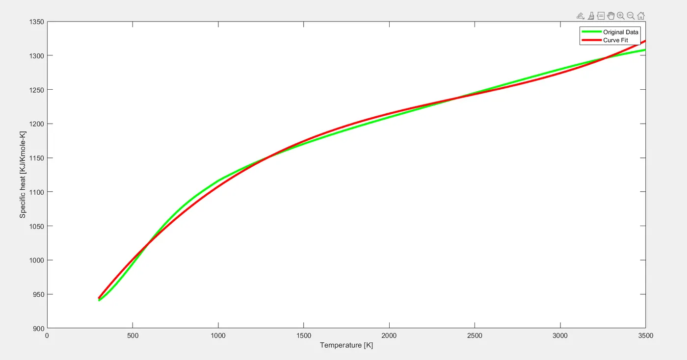
Figure02: Curve fitting for cubic polynomial.

Detailed explanation of program-02:

1. Name of Program, “Programming the Curve fitting of Cubic polynomial for a given data”.
3. Clears your workspace.
4. Closes all the figures.
5. Clears Command window.
7. % Preparing data

No we are loading the data so we can use it for the study.

8. Cp_data = load('data');

For loading the data we are using the load command using which we are loading the data under the variable ‘Cp_data’.

9. temp = Cp_data(:,1);

Here, we are simply selecting the column one of the data [Cp_data(:,1)] and as the data is for the independent variable temperature we are assigning the variable ‘temp’ for it.

10. Cp = Cp_data(:,2);

Here, we are simply selecting the column two of the data [Cp_data(:,2)] and as the data is for the function i.e. specific heat we are assigning the variable ‘Cp’ for it.

12. % Curve Fit for linear equation.
13. % Cp = ax^3 + bx^2 + cx + d
14. Coeff = polyfit(temp,Cp,3);

There is a inbuilt command in matlab for the curve fitting of the available data i. e. polyfit command. By using this command we find values of coefficients for the best fit of the function equation. Therefoe the variable “coeff’ is used. Here temp and Cp represents the the values of the column-01 and column-2 resp. of the data set for which the curve fitting needs to be done. And number 3 represents the order of the polynomial, for cubic equation it’s three.

15. Predicted_Cp = polyval(Coeff,temp);

Now we are fitting curve beyond the observed data points (Extrapolation) for that we need to determine the predicted values of a function by using polyval command.  Therefore the variable ‘Predicted_Cp’ is used and values of coefficients (coeff) and the independent variable (temp) were used as input credentials to execute the command.

17. % Plotting
18. plot(temp,Cp,'linewidth',3,'color','g');

Plotting the curve for function and it’s independent variable of the data set by using plot command and required input credentials.

19. % Compare my curve fit
20. hold on
21. plot(temp,Predicted_Cp,'linewidth',3,'color','r')

Plotting the curve for the predicted values of the function and the given values of the independent variable by using plot command and required input credentials.

23. xlabel('Temperature [K]');
24. ylabel('Specific heat [KJ/Kmole-K]');

Labelling X and Y axis..

25. legend('Original Data','Curve Fit');

Defining the legends for the convenient study of the plots.

Program-03:
Curve fitting of a linear polynomial by splitting the data into different ranges:
01.	% Programming the Curve fitting of Linear polynomial for a given data.
02.	
03.	clear all
04.	close all
05.	clc
06.	
07.	% Preparing data
08.	
09.	Data = load('data');
10.	n = length(Data);
11.	
12.	% Splitting Data into iterations.
13.	
14.	s = 10
15.	a = 1
16.	b = n/s
17.	
18.	% Assigning values for temperature and Specific heat.
19.	
20.	for i = 1:s
21.	
22.	temp = Data(a:b,1);
23.	cp = Data(a:b,2);
24.	
25.	% Executung the curve fitting commands for Linear polynomial.
26.	
27.	coeff = polyfit(temp,cp,1);
28.	P_cp = polyval(coeff,temp);
29.	
30.	% plotting predicted curve.
31.	plot(temp,cp,'linewidth',4,'color','r');
32.	hold on
33.	plot(temp,P_cp,'linewidth',3,'color','g');
34.	
35.	a = b;
36.	b = b + n/s;
37.	
38.	xlabel('Temperature [k]');
39.	ylabel('Specific heat [KJ/Kmole-K]');
40.	legend('Original Data','Curve Fit');
41.	end

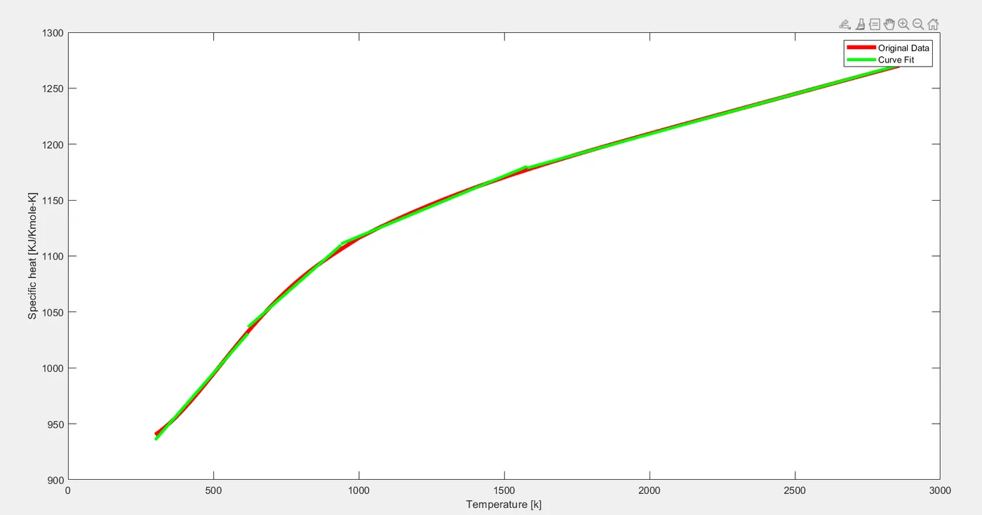
Figure03: Curve fitting for linear polynomial by splitting the data into number of data sets.

Detailed explanation of program-03:

1. Name of Program, “Programming the Curve fitting of linear polynomial for a given data by splitting it into different ranges”.
3. Clears your workspace.
4. Closes all the figures.
5. Clears Command window.
7. % Preparing data
9. Data = load('data');

No we are loading the data so we can use it for the study.

10. n = length(Data);

Assigning the variable ‘n’ for the length of data which is under consideration for the study. Command ‘length’ executes all the values of the ‘Data’.

            i.e. n  = Total number of values of the data.

12. % Splitting Data into iterations.

There are two ways in which we can choose the best fit for the plotted curve:

1. Change the order of the polynomial greater the order better the fit.
2. Split the data into different ranges and plot the curve individually for each range of the data.

In order to split the data in matlab we need program the the ranges of the data for which we will have draw the curve.

14. s = 10

Here the variable ‘s’ is used by assigning the value to it as per our data’s requirements, so that later it can be used to define the other variables in the program. 

15. a = 1

If we are going to split the data into different ranges then for every range there will be a different initial value and final value of the data. Now for Range-01 consider the initial value as variable ‘a’ i.e. 1 and final value as variable ‘b’ i.e. n/s.

16. b = n/s

b = final value for the range. Defined as n/s.

18. % Assigning values for temperature and Specific heat.
20. for i = 1:s

Starting the for loop by assigning the variable ‘i’ values from 1 to 10 (s).

22. temp = Data(a:b,1);

Selecting values of the temperature for the particular range in consideration. For temperature the values will be taken into consideration will be from a to b of column-I.

23. cp = Data(a:b,2);

            Selecting values of the specific heat for the particular range in consideration. For

            Specific heat the values will be taken into consideration will be from a to b of column-II.

24. % Executung the curve fitting commands for Linear polynomial.
26. coeff = polyfit(temp,cp,1);

Assigning the variable ‘coeff’ which will hold the outcomes of the command ‘polyfit’. ‘polyfit’is the inbuilt command in matlab which will give us the values of the coefficients of the function polynomial (Values of coefficients a and b) for the best fit of the curve. Input credentials for the ‘polyfit’ command are: Independent variable (temp), Function (Cp) and Order of the polynomial (Linear = 1).

28. P_cp = polyval(coeff,temp);

Now for extrapolation we will need the predicted values of the function (Cp), so we can draw the curve for the points beyond the observed data. Thus to obtain the values of the predicted Cp we are using the inbuilt command ‘polyval’ which will give us the values of the predicted functions. Coefficients and the temperatures are the input credentials for the command ‘polyval’.

30. % Comparing the Curve Fit.
31. plot(temp,cp,'linewidth',4,'color','r');

Plotting the curve for the data used.

32. hold on
33. plot(temp,P_cp,'linewidth',3,'color','g');

Plotting the curve for the predicted values of the function (Cp).

35. a = b;

Redefining the initial value (a) for the next range.

36. b = b + n/s;

Redefining the final value (b) for the next range.

37. xlabel('Temperature [k]');
38. ylabel('Specific heat [KJ/Kmole-K]');

Labeling the X and Y axis of the plot.

40. legend('Original Data','Curve Fit');

Defining the legends for the both curves.

41. end

End of for loop.

Program-04:
Curve fitting of a cubic polynomial by splitting the data into different ranges:
01.	% Programming the Curve fitting of Cubic polynomial for a given data.
02.	
03.	clear all
04.	close all
05.	clc
06.	
07.	% Preparing data
08.	
09.	Data = load('data');
10.	n = length(Data);
11.	
12.	% Splitting Data into iterations.
13.	
14.	s = 10
15.	a = 1
16.	b = n/s
17.	
18.	% Assigning values for temperature and Specific heat.
19.	
20.	for i = 1:s
21.	
22.	temp = Data(a:b,1);
23.	cp = Data(a:b,2);
24.	
25.	% Executing the curve fitting commands for Cubic polynomial.
26.	
27.	coeff = polyfit(temp,cp,3);
28.	P_cp = polyval(coeff,temp);
29.	
30.	% plotting predicted curve.
31.	plot(temp,cp,'linewidth',4,'color','r');
32.	hold on
33.	plot(temp,P_cp,'linewidth',3,'color','g');
34.	
35.	a = b;
36.	b = b + n/s;
37.	
38.	xlabel('Temperature [k]');
39.	ylabel('Specific heat [KJ/Kmole-K]');
40.	legend('Original Data','Curve Fit');
41.	end

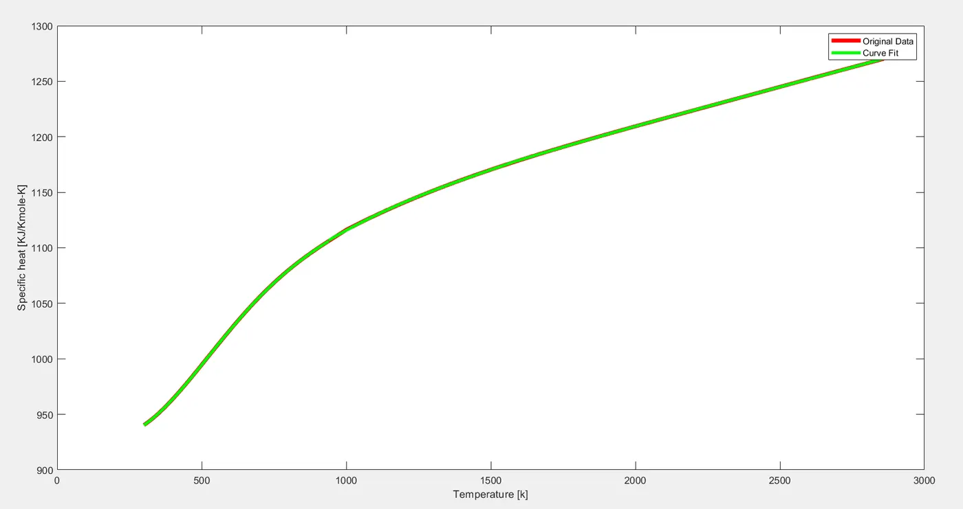
Figure04: Curve fitting for cubic polynomial by splitting the data into number of data sets.

Detailed explanation of program-04:

1. Name of Program, “Programming the Curve fitting of cubic polynomial for a given data by splitting it into different ranges”.
3. Clears your workspace.
4. Closes all the figures.
5. Clears Command window.
7. % Preparing data
9. Data = load('data');

No we are loading the data so we can use it for the study.

10. n = length(Data);

Assigning the variable ‘n’ for the length of data which is under consideration for the study. Command ‘length’ executes all the values of the ‘Data’.

            i.e. n  = Total number of values of the data.

12. % Splitting Data into iterations.

There are two ways in which we can choose the best fit for the plotted curve:

1. Change the order of the polynomial greater the order better the fit.
2. Split the data into different ranges and plot the curve individually for each range of the data.

In order to split the data in matlab we need program the the ranges of the data for which we will have draw the curve.

14. s = 10

Here the variable ‘s’ is used by assigning the value to it as per our data’s requirements, so that later it can be used to define the other variables in the program. 

15. a = 1

If we are going to split the data into different ranges then for every range there will be a different initial value and final value of the data. Now for Range-01 consider the initial value as variable ‘a’ i.e. 1 and final value as variable ‘b’ i.e. n/s.

16. b = n/s

b = final value for the range. Defined as n/s.

18. % Assigning values for temperature and Specific heat.
20. for i = 1:s

Starting the for loop by assigning the variable ‘i’ values from 1 to 10 (s).

22. temp = Data(a:b,1);

Selecting values of the temperature for the particular range in consideration. For temperature the values will be taken into consideration will be from a to b of column-I.

23. cp = Data(a:b,2);

            Selecting values of the specific heat for the particular range in consideration. For

            Specific heat the values will be taken into consideration will be from a to b of column-II. 

24. % Executung the curve fitting commands for Linear polynomial.
26. coeff = polyfit(temp,cp,3);

Assigning the variable ‘coeff’ which will hold the outcomes of the command ‘polyfit’. ‘polyfit’is the inbuilt command in matlab which will give us the values of the coefficients of the function polynomial (Values of coefficients a and b) for the best fit of the curve. Input credentials for the ‘polyfit’ command are: Independent variable (temp), Function (Cp) and Order of the polynomial (Cubic = 3).

28. P_cp = polyval(coeff,temp);

Now for extrapolation we will need the predicted values of the function (Cp), so we can draw the curve for the points beyond the observed data. Thus to obtain the values of the predicted Cp we are using the inbuilt command ‘polyval’ which will give us the values of the predicted functions. Coefficients and the temperatures are the input credentials for the command ‘polyval’.

30. % Comparing the Curve Fit.
31. plot(temp,cp,'linewidth',4,'color','r');

Plotting the curve for the data used. 

32. hold on
33. plot(temp,P_cp,'linewidth',3,'color','g');

Plotting the curve for the predicted values of the function (Cp).

35. a = b;

Redefining the initial value (a) for the next range.

36. b = b + n/s;

Redefining the final value (b) for the next range.

38. xlabel('Temperature [k]');
39. ylabel('Specific heat [KJ/Kmole-K]');

Labeling the X and Y axis of the plot.

40. legend('Original Data','Curve Fit');

Defining the legends for the both curves.

41. end 

           End of for loop.

Errors occurred during programming are as follows:

1. Error:

Value of ‘b’ for each incremented data set is not defined correctly.

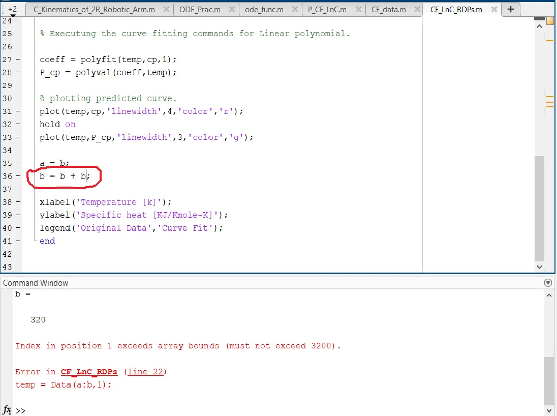
Figure05: Value of ‘b’ is not correctly defined.

Correction:

                  The length of each data set is of 320 units, therefore the value of final data point (value of b)  must get incremented by 320 units. But here by mistake we defined ‘b = b + b’ and value of ‘b’ changes for each loop and by the end of last loop the value of ‘b’ crosses the total number of data units in consideration. Therefore to eliminate the error we need to define ‘b’ such that it will take the final value of next data set. (b = b + n/s)

Conclusion:

In this section we studied the curve fitting for the polynomials of different orders. From study we came to know that the values of the function of the independent variable for the particular phenomenon can be predicted for the best fit of the polynomial using curve fitting.

To obtain the best fit for the set of data into the consideration we must divide the data into equal number of data sets and plot the curve for each data set individually.

We also learn the programming of the curve fitting in matlab which makes the study of the curve fit easy and convenient to understand.

Question-01:

How to make a curve fit perfectly?

Answer:

To make a perfect curve following step must be followed:

1. Take a set of data under consideration and divide it into equal number of data sets.
2. Now for each data set calculate the values of the coefficients of the mathematical function.
3. Now calculate the predicted values of the function for that particular data set.
4. Finally by using the values of coefficients and predicted values of the function we can draw the curve fit for that particular data set.
5. Follow the same procedure for remaining number of data sets.
6. This procedure of plotting the curve is known as split fit, in which the dat is aplitted into various data sets.

Question-02

How to get the best fit?

Answer:

The mathematical function for which we are plotting the curve consists of polynomial and it’s order.

After plotting the curve for a particular data, we also need to plot the fitting curve for the same independent variable having predicted values of the function.

By determining the values of the coefficients and the predicted values of the function we can plot the curve. While plotting the order of the polynomial plays a vital role:

If the polynomial is of first order (Linear) that means it has two points through which the curve will get plotted results in less accurate fit.

Whereas if the order of the polynomial is two (Quadratic) there will be three points through which the curve will pass making the curve more accurate.

As the order of polynomial increases accuracy of the fit of curve increases.

Therefore to select the best fit of the curve we must choose the order of the polynomial accordingly.

Question-03

What must be done to improve cubic fit?

Answer:

To improve cubic curve following step must be followed:

1. Take a set of data under consideration and divide it into equal number of data sets.
2. Now for each data set calculate the values of the coefficients of the mathematical function.
3. Now calculate the predicted values of the function for that particular data set.
4. Finally by using the values of coefficients and predicted values of the function we can draw the curve fit for that particular data set.
5. Follow the same procedure for remaining number of data sets.
6. This procedure of plotting the curve is known as split fit, in which the data is splited into various data sets.