CALCULATION OF ADIABATIC FLAME TEMPERATURE FOR DIFFERENT HYDRO CARBONS IN CONSTANT PRESSURE AND VOLUME CHAMBERS AND EXAMINING THE EFFECT OF EQUIVALANCE RATIO, BOND STRENGTH AND NO OF CARBON ATOMS ON ADIABATIC FLAME TEMPERATURE USING PYTHON AND CANTERA
Aim :
1) To calculate Adiabatic flame temperature of a given species in a constant volume combustion chamber
2) To calculate Adiabatic flame temperature of a given species in a constant pressure combustion chamber (considering the effect of product at initial reactant temperature)
3) Examining the effect of bond strength and no of carbon atoms on Adiabatic flame temperature
Introduction :
For designing any combustion chamber whether a constant volume type or a constant pressure(steady flow) type as in gas turbines, maximum temperature attained has been kept below keeping a note of metallurgical considerations of parts in chamber. The maximum temperature can be attained only when all of heat relerased is used to increase temperatutre of products. The maximum temperature is called Adiabatic flame temperature. This temperature is dependent on Air-Fuel ratio , type of fuel used and type of combustion chamber
Theory :
For a given combustion device, say a piston engine, how much fuel and air should be injected in order to completely burn both? This question can be answered by balancing the combustion reaction equation for a particular fuel. A stoichiometric mixture contains the exact amount of fuel and oxidizer such that after combustion is completed, all the fuel and oxidizer are consumed to form products. This ideal mixture approximately yields the maximum flame temperature, as all the energy released from combustion is used to heat the products.
Combustion stoichiometry for a general hydrocarbon fuel, with air can be expressed as

The amount of air required for combusting a stoichiometric mixture is called stoichiometric or theoretical air. The above formula is for a single-component fuel and cannot be applied to a fuel consisting of multiple components.
In practice, fuels are often combusted with an amount of air different from the stoichiometric ratio. If less air than the stoichiometric amount is used, the mixture is described as fuel rich. If excess air is used, the mixture is described as fuel lean. For this reason, it is convenient to quantify the combustible mixture using one of the following commonly used methods
Fuel-Air Ratio (FAR): The fuel-air ratio, f, is given by

where mf and ma are the respective masses of the fuel and the air. For a stoichiometric mixture
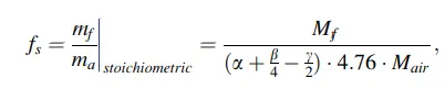
where Mf and Mair (~28.84 kg/kmol) are the average masses per mole of fuel and air,
respectively. The range of f is bounded by zero and 1. Most hydrocarbon fuels have a stoichiometric fuel-air ratio, fs, in the range of 0.05–0.07.
Equivalence Ratio: Normalizing the actual fuel-air ratio by the stoichiometric fuelair ratio gives the equivalence ratio, f.
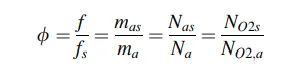
The subscript s indicates a value at the stoichiometric condition. Φ <1 is a lean mixture, Φ= 1 is a stoichiometric mixture, and Φ >1 is a rich mixture. Similar to f, the range of Φ is bounded by zero and infinite corresponding to the limits of pure air and fuel respectively. Note that equivalence ratio is a normalized quantity that provides the information regarding the content of the combustion mixture.
assuming that the products contain major species only (complete combustion) and excess air, the global equation for lean combustion Φ<=1 is
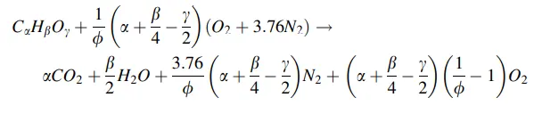
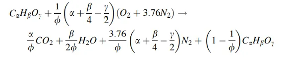
For rich combustion (Φ>1), the products may contain CO, unburned fuels, and other species formed by the degradation of the fuel. Often additional information on the products is needed for complete balance of the chemical reaction. If the products are assumed to contain only unburned fuel and major combustion products, the corresponding global equation can be written as
constant volume chamber :
The volume of the chamber before and after combustion remains same so 1st law of thermodynamics is applied
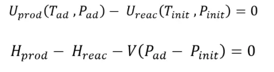
Using Ideal gas :

since there is no path for heat to be released,H2o vapours will not condense, Thus we will only get lower heating value (LHV)
constant pressure chamber :
This is useful for combustion gas turbines.The flow of air and fuel is continous and there is change in pressure due to combustion and expansion
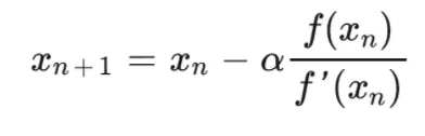
The governing equation is

In a constant pressure chamber , some part of heat released is used to perform work of expansion of volume to keep pressure constant . This is the reason Adiabatic flame temperature in constant pressure chamber is less than in constant volume chamber
Higher and lower heating values :
If during combustion the reactants at STP are burned to form products,there is release of heat . This heat value is called Lower heating value. when a gas is cooled it releases heat , if the gaseous products are cooled more heat is released along with LHV . This total heat released is called HHV

Newton Raphson solver :
The equations written above are solved using Newton Raphson solver . This solver starts from a guess value and using curves slope at guess value it guesses new value which has less curve slope , In this way minima point is reached .This iterative process continues till the difference in slope becomes less than the tolerance value
Adiabatic flame temperature calculation in Constant pressure with heat loss :
'''
 program to calculate Adaibatic flame temperature for different HydroCarbon combustion in constant pressure chamber with heat loss for different equivalence ratios

 lean combustion equation (phi < 1)

 CaHbOd + (1/phi)(a+b/4-d/2) (O2 + 3.76 N2) ------>  a CO2 + b/2 H2O + (3.76/phi)(a+b/4-d/2) N2 + (1/phi - 1)(a+b/4-d/2) O2

Rich combustion equation (phi > 1)

For rich combustion (phi>1), the products may contain CO, unburned fuels, and other species formed by the degradation of the fuel. Often additional information on the products is needed for complete balance of the chemical reaction. If the products are assumed to contain only unburned fuel and major combustion products, the corresponding global equation can be written as

CaHbOd + (1/phi)(a+b/4-d/2) (O2 + 3.76 N2) ------> (a/phi) CO2 + (b/2*phi) H2O + (3.76/phi)(a+b/4-d/2) N2 + (1 - 1/phi) CH4

Stoichiometric combustion (phi =1)

 CaHbOd + (a+b/4-d/2) (O2 + 3.76 N2) ------>  a CO2 + b/2 H2O + 3.76(a+b/4-d/2) N2

Author : Harshith Rajamahanti

'''
import matplotlib.pyplot as plt
import math

#Function for calculating enthalpy

def h(T,coeffs):

	R=8.314 #j/mol-K

	a1=coeffs[0]
	a2=coeffs[1]
	a3=coeffs[2]
	a4=coeffs[3]
	a5=coeffs[4]
	a6=coeffs[5]

	return (a1+a2*T/2+a3*pow(T,2)/3+a4*pow(T,3)/4+a5*pow(T,4)/5+a6/T)*R*T

CH4_coeffs_l=[5.14987613E+00,-1.36709788E-02, 4.91800599E-05, -4.84743026E-08, 1.66693956E-11, -1.02466476E+04, -4.64130376E+00]

C2H6_coeffs_l=[4.29142492E+00, -5.50154270E-03, 5.99438288E-05, -7.08466285E-08, 2.68685771E-11, -1.15222055E+04, 2.66682316E+00]

C2H4_coeffs_l=[3.95920148E+00, -7.57052247E-03, 5.70990292E-05, -6.91588753E-08, 2.69884373E-11, 5.08977593E+03, 4.09733096E+00]

C2H2_coeffs_l=[8.08681094E-01, 2.33615629E-02, -3.55171815E-05, 2.80152437E-08, -8.50072974E-12, 2.64289807E+04, 1.39397051E+01]

O2_coeffs_l=[3.78245636E+00, -2.99673416E-03, 9.84730201E-06, -9.68129509E-09, 3.24372837E-12, -1.06394356E+03, 3.65767573E+00 ]

N2_coeffs_l=[0.03298677E+02, 0.14082404E-02, -0.03963222E-04, 0.05641515E-07, -0.02444854E-10, -0.10208999E+04, 0.03950372E+02 ]

CO2_coeffs_h=[3.85746029E+00, 4.41437026E-03, -2.21481404E-06, 5.23490188E-10, -4.72084164E-14, -4.87591660E+04, 2.27163806E+00]

H2O_coeffs_h=[3.03399249E+00, 2.17691804E-03, -1.64072518E-07, -9.70419870E-11, 1.68200992E-14, -3.00042971E+04, 4.96677010E+00]

N2_coeffs_h=[0.02926640E+02, 0.14879768E-02, -0.05684760E-05, 0.10097038E-09, -0.06753351E-13, -0.09227977E+04, 0.05980528E+02]

O2_coeffs_h=[3.28253784E+00, 1.48308754E-03, -7.57966669E-07, 2.09470555E-10, -2.16717794E-14, -1.08845772E+03, 5.45323129E+00]

CH4_coeffs_h=[2.28571772E+00, 7.23990037E-03, -2.98714348E-06, 5.95684644E-10, -4.67154394E-14, 1.67755843E+04, 8.48007179E+00]

C2H6_coeffs_h=[1.07188150E+00, 2.16852677E-02, -1.00256067E-05, 2.21412001E-09, -1.90002890E-13, -1.14263932E+04, 1.51156107E+01]

C2H4_coeffs_h=[2.03611116E+00, 1.46454151E-02, -6.71077915E-06, 1.47222923E-09, -1.25706061E-13, 4.93988614E+03, 1.03053693E+01]

C2H2_coeffs_h=[4.14756964E+00, 5.96166664E-03, -2.37294852E-06, 4.67412171E-10, -3.61235213E-14, 2.59359992E+04, -1.23028121E+00]

case=2

#Defining the function by root solving by Newton raphson method

a=1
b=4
d=0

def f(T,phi,hloss):

	T_stp=298.15
	R=8.314 #j/mol-K


	if (d==0):

		if (a==1) and (b==4):
			fuel_h_r=h(T_stp,CH4_coeffs_l)
			fuel_h_p=h(T,CH4_coeffs_h)
			fuel_h_p_stp=h(T_stp,CH4_coeffs_h)

		if (a==2):
			if (b==2):
				fuel_h_r=h(T_stp,C2H2_coeffs_l)
				fuel_h_p=h(T,C2H2_coeffs_h)
				fuel_h_p_stp=h(T_stp,C2H2_coeffs_h)

			if(b==4):
				fuel_h_r=h(T_stp,C2H4_coeffs_l)
				fuel_h_p=h(T,C2H4_coeffs_h)
				fuel_h_p_stp=h(T_stp,C2H4_coeffs_h)

			if(b==6):
				fuel_h_r=h(T_stp,C2H6_coeffs_l)
				fuel_h_p=h(T,C2H6_coeffs_h)
				fuel_h_p_stp=h(T_stp,C2H6_coeffs_h)

	h_CO2_p=h(T,CO2_coeffs_h)

	h_CO2_p_stp=h(T_stp,CO2_coeffs_h)

	h_N2_p=h(T,N2_coeffs_h)

	h_N2_p_stp=h(T_stp,N2_coeffs_h)

	h_H2O_p=h(T,H2O_coeffs_h)

	h_H2O_p_stp=h(T_stp,H2O_coeffs_h)

	h_O2_p=h(T,O2_coeffs_h)

	h_O2_p_stp=h(T_stp,O2_coeffs_h)

	if phi <=1:
		H_products= a*h_CO2_p + (b/2)*h_H2O_p + (3.76/phi)*(a+b/4-d/2)*h_N2_p + (a+b/4-d/2)*(1/phi - 1)*h_O2_p
		H_products_stp= a*h_CO2_p_stp + (b/2)*h_H2O_p_stp + (3.76/phi)*(a+b/4-d/2)*h_N2_p_stp + (a+b/4-d/2)*(1/phi - 1)*h_O2_p_stp


	elif phi >1:
		H_products=(a/phi)*h_CO2_p + (b/(2*phi))*h_H2O_p + (3.76/phi)*(a+b/4-d/2)*h_N2_p + (1 - 1/phi)*fuel_h_p
		H_products_stp=(a/phi)*h_CO2_p_stp + (b/(2*phi))*h_H2O_p_stp + (3.76/phi)*(a+b/4-d/2)*h_N2_p_stp + (1 - 1/phi)*fuel_h_p_stp


	h_O2_r=h(T_stp,O2_coeffs_l)

	h_N2_r=h(T_stp,N2_coeffs_l)

	H_reactants= (1*fuel_h_r) + (1/phi)*(a+b/4-d/2)*h_O2_r + (3.76/phi)*(a+b/4-d/2)*h_N2_r


	return (H_products - H_reactants) - hloss*(H_products_stp - H_reactants)

def fprime(T,phi,hloss):

	return (f(T+1e-6,phi,hloss)-f(T,phi,hloss))/(1e-6)

if case==1:

	# Defining Newton Raphson solver

	alpha=0.2

	tol=1e-4

	iter=0

	T_guess=1500

	phi_min=0.1

	phi_max=2

	phi_diff=0.1

	phi_num=int(round((phi_max-phi_min)/phi_diff))

	phi=[]

	hloss=0

	for i in range(0,phi_num+1):
		phi.append(round((((i)*phi_diff)+phi_min),3))

	AFT_py=[]
	iteration=[]

	for cter in range(0,len(phi)):

		while (abs(f(T_guess,phi[cter],hloss)) > tol):
			T_guess=T_guess-(f(T_guess,phi[cter],hloss)/fprime(T_guess,phi[cter],hloss))*alpha
			iter=iter+1


		iteration.append(iter)
		AFT_py.append(T_guess)


	# Solution using Cantera

	import cantera
	gas = cantera.Solution('gri30.cti')
	AFT_cant=[]

	if (a==1) and (b==4):
		species='Ch4'
	if (a==2):
		if (b==6):
			species='C2H6'
		if (b==4):
			species='C2H4'
		if (b==2):
			species='C2H2'

	for j in range(0,len(phi)):
		gas.TPX=298.15,101325,{species:1,'O2':(1/phi[j])*(a+b/4-d/2),'N2':(3.76/phi[j])*(a+b/4-d/2)}
		gas.equilibrate('hp','auto')
		AFT_cant.append(gas.T)

	print(AFT_cant)
	print(AFT_py)
	print(iteration)
	plt.plot(phi,AFT_py,'-o',color='blue',label='Python')
	plt.plot(phi,AFT_cant,'-o',color='red',label='Cantera')
	plt.xlabel('Equivalence Ratio',fontsize=14)
	plt.ylabel('Adiabatic Flame Temp in K',fontsize=14)
	plt.legend()
	plt.title('Adiabatic flame temperature of %s at different Equivalence Ratios in a constant pressure chamber'% species,fontweight='bold')
	plt.grid('on')
	plt.show()

	plt.plot(phi,iteration)
	plt.xlabel('Equivalence Ratio',fontsize=14)
	plt.ylabel('Number of Iterations',fontsize=14)
	plt.title(' %s Number of Iterations in Newton Raphson for AFT calculation vs Equivalence Ratio' % species)
	plt.show()

	print(species)

if case==2:
	# Defining Newton Raphson solver

	if (a==1) and (b==4):
		species='Ch4'
	if (a==2):
		if (b==6):
			species='C2H6'
		if (b==4):
			species='C2H4'
		if (b==2):
			species='C2H2'

	alpha=0.2

	tol=1e-4

	iter=0

	T_guess=1500

	hloss_min=0

	hloss_max=1

	hloss_diff=0.05

	hloss_num=int(round((hloss_max-hloss_min)/hloss_diff))

	hloss=[]


	for i in range(0,hloss_num+1):
		hloss.append(round((((i)*hloss_diff)+hloss_min),3))
	phi=1

	T_hloss=[]
	iteration=[]

	for cter in range(0,len(hloss)):

		while (abs(f(T_guess,phi,hloss[cter])) > tol):
			T_guess=T_guess-(f(T_guess,phi,hloss[cter])/fprime(T_guess,phi,hloss[cter]))*alpha
			iter=iter+1


		iteration.append(iter)
		T_hloss.append(T_guess)


	print(T_hloss)
	print(iteration)
	plt.plot(hloss,T_hloss,'-o',color='blue',label='Python')
	plt.xlabel('Heat loss factor',fontsize=14)
	plt.ylabel('Adiabatic Flame Temp in K',fontsize=14)
	plt.legend()
	plt.title('Adiabatic flame temperature of %s at different heat loss factors' % species,fontweight='bold')
	plt.grid('on')
	plt.show()

	plt.plot(hloss,iteration)
	plt.xlabel('heat loss factor',fontsize=14)
	plt.ylabel('Number of Iterations',fontsize=14)
	plt.title('Number of Iterations for %s in Newton Raphson for AFT calculation vs heat loss factor'% species)
	plt.show()
code explanation :
The above code consists of two cases. Case 1 deals with how the adiabatic flame temperature varies wrt to Equivalance ratio for different Hydro carbons with a fixed heat loss factor where as Case 2 deals with how the AFT varies wrt to heat loss factor
steps :
- Consediring the Example of Methane for better understanding of the code
- CH4 + 2(O2+3.76N2) ---------> CO2 + 2H2O + 7.52 N2 (Stoichiometric case)
- Enthalpy H is a function of Temperature and Coefficients
- The coefficients are taken from NASA polynomial data which is chemkin II data
- After collecting the coefficients data the enthalpy is calculated in terms of Temperature
- H=(a1 + a2/2 T + a3/3 T^2 + a4/4 T^3 + a5/5 T^4 +a6/T) RT
- The NASA data file contains 14 coefficients for each and every species from which the first 7 represent high temperatute coefficents and last 7 represent low temperature coefficients, Depending on the local temperature ranges the co efficient data is taken
- Considering the gas to be ideal so the enthalpy is only the function of temperature
- Enthalpy of products and reactants are calculated in terms of temperature and use the equation dH = 0
- Now An polynomial equation is obtained in terms of Temperature which has to be solved for the T value which in turn gives the Adiabatic flame temperature value
- Newton Raphson method is used to solve for the T value
Python code steps :
- At first Important library files are inclued and the comments are written in ''' '''
- Enthalpy function h is taken in terms of Coefficients and Temperature
- Coefficients values are obtained from NASA polynomial data file
- So the function h returns the polynomial interms of temperature only
- A function f is taken interms of phi, temperature and hloss factor
- Now the derivative of the function f is evaluated using fprime function
Case 1 : Variation of AFT wrt to Equivalence ratio
- Here hloss factor valued is fixed and a set of phi values are considered in order to examine how AFT is varied wrt to phi
- phi values are taken from 0.1 to 2 with interval of 0.1
- Newton Raphson solver code is run in a loop for different phi values and AFT is calculated at each phi value
- Later the same code is written by importing cantera and AFT is calculated at different phi values
Case 2 : variation of AFT wrt to hloss factor
- Here phi valued is fixed and a set of hloss factor values are considered in order to examine how AFT is varied wrt to hloss factor
- hloss factor values are taken from 0 to 1 with an interval of 0.05
- Newton Raphson solver code is run in a loop for different hloss factor values and AFT is calculated at each hloss factor value
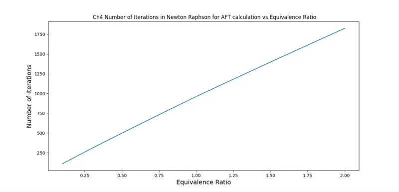
Later the values for AFT in cantera code and python code are compared in a graph and how the iterations for solving the temperature in newton raphson method is varied wrt to changes in phi and hloss factors is also observed
Outputs :
For lean mixture

For Rich mixture

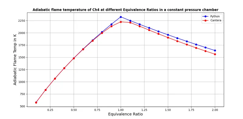
Considering Methane i.e a=1; b=4; and d=0
Case 1 :
Case 2 :
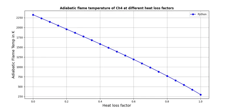
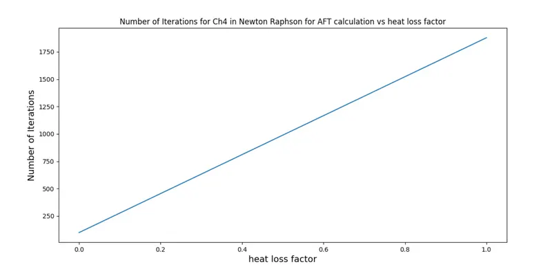
similarly the plots can be generated for different hydro carbons by changing the a b and d values in the above code
Adiabatic flame temperature calculation in Constant volume chamber :
'''
 program to calculate Adaibatic flame temperature for different HydroCarbon combustion in constant volume chamber for different equivalence ratios and also  calculating variation of AFT wrt to variation of carbon atoms and hydrogen atoms

 lean combustion equation (phi < 1)

 CaHbOd + (1/phi)(a+b/4-d/2) (O2 + 3.76 N2) ------>  a CO2 + b/2 H2O + (3.76/phi)(a+b/4-d/2) N2 + (1/phi - 1)(a+b/4-d/2) O2

Rich combustion equation (phi > 1)

For rich combustion (phi>1), the products may contain CO, unburned fuels, and other species formed by the degradation of the fuel. Often additional information on the products is needed for complete balance of the chemical reaction. If the products are assumed to contain only unburned fuel and major combustion products, the corresponding global equation can be written as

CaHbOd + (1/phi)(a+b/4-d/2) (O2 + 3.76 N2) ------> (a/phi) CO2 + (b/2*phi) H2O + (3.76/phi)(a+b/4-d/2) N2 + (1 - 1/phi) CH4

Stoichiometric combustion (phi =1)

 CaHbOd + (a+b/4-d/2) (O2 + 3.76 N2) ------>  a CO2 + b/2 H2O + 3.76(a+b/4-d/2) N2

Author : Harshith Rajamahanti

'''
import matplotlib.pyplot as plt
import math

#Function for calculating enthalpy

def h(T,coeffs):

	R=8.314 #j/mol-K

	a1=coeffs[0]
	a2=coeffs[1]
	a3=coeffs[2]
	a4=coeffs[3]
	a5=coeffs[4]
	a6=coeffs[5]

	return (a1+a2*T/2+a3*pow(T,2)/3+a4*pow(T,3)/4+a5*pow(T,4)/5+a6/T)*R*T

CH4_coeffs_l=[5.14987613E+00,-1.36709788E-02, 4.91800599E-05, -4.84743026E-08, 1.66693956E-11, -1.02466476E+04, -4.64130376E+00]

C2H6_coeffs_l=[4.29142492E+00, -5.50154270E-03, 5.99438288E-05, -7.08466285E-08, 2.68685771E-11, -1.15222055E+04, 2.66682316E+00]

C2H4_coeffs_l=[3.95920148E+00, -7.57052247E-03, 5.70990292E-05, -6.91588753E-08, 2.69884373E-11, 5.08977593E+03, 4.09733096E+00]

C2H2_coeffs_l=[8.08681094E-01, 2.33615629E-02, -3.55171815E-05, 2.80152437E-08, -8.50072974E-12, 2.64289807E+04, 1.39397051E+01]

C3H8_coeffs_l=[0.93355381E+00, 0.26424579E-01, 0.61059727E-05, -0.21977499E-07, 0.95149253E-11, -0.13958520E+05, 0.19201691E+02]

O2_coeffs_l=[3.78245636E+00, -2.99673416E-03, 9.84730201E-06, -9.68129509E-09, 3.24372837E-12, -1.06394356E+03, 3.65767573E+00 ]

N2_coeffs_l=[0.03298677E+02, 0.14082404E-02, -0.03963222E-04, 0.05641515E-07, -0.02444854E-10, -0.10208999E+04, 0.03950372E+02 ]

CO2_coeffs_h=[3.85746029E+00, 4.41437026E-03, -2.21481404E-06, 5.23490188E-10, -4.72084164E-14, -4.87591660E+04, 2.27163806E+00]

H2O_coeffs_h=[3.03399249E+00, 2.17691804E-03, -1.64072518E-07, -9.70419870E-11, 1.68200992E-14, -3.00042971E+04, 4.96677010E+00]

N2_coeffs_h=[0.02926640E+02, 0.14879768E-02, -0.05684760E-05, 0.10097038E-09, -0.06753351E-13, -0.09227977E+04, 0.05980528E+02]

O2_coeffs_h=[3.28253784E+00, 1.48308754E-03, -7.57966669E-07, 2.09470555E-10, -2.16717794E-14, -1.08845772E+03, 5.45323129E+00]

CH4_coeffs_h=[2.28571772E+00, 7.23990037E-03, -2.98714348E-06, 5.95684644E-10, -4.67154394E-14, 1.67755843E+04, 8.48007179E+00]

C2H6_coeffs_h=[1.07188150E+00, 2.16852677E-02, -1.00256067E-05, 2.21412001E-09, -1.90002890E-13, -1.14263932E+04, 1.51156107E+01]

C2H4_coeffs_h=[2.03611116E+00, 1.46454151E-02, -6.71077915E-06, 1.47222923E-09, -1.25706061E-13, 4.93988614E+03, 1.03053693E+01]

C2H2_coeffs_h=[4.14756964E+00, 5.96166664E-03, -2.37294852E-06, 4.67412171E-10, -3.61235213E-14, 2.59359992E+04, -1.23028121E+00]

C3H8_coeffs_h=[0.75341368E+01, 0.18872239E-01, -0.62718491E-05, 0.91475649E-09, -0.47838069E-13, -0.16467516E+05, -0.17892349E+02]

case=2

if case==1: #variation of AFT wrt to phi for different Hydro carbons

	#Defining the function by root solving by Newton raphson method

	a=2
	b=6
	d=0

	def f(T,phi):

		T_stp=298.15
		R=8.314 #j/mol-K


		if (d==0):

			if (a==1) and (b==4):
				fuel_h_r=h(T_stp,CH4_coeffs_l)
				fuel_h_p=h(T,CH4_coeffs_h)

			if (a==2):
				if (b==2):
					fuel_h_r=h(T_stp,C2H2_coeffs_l)
					fuel_h_p=h(T,C2H2_coeffs_h)

				if(b==4):
					fuel_h_r=h(T_stp,C2H4_coeffs_l)
					fuel_h_p=h(T,C2H4_coeffs_h)

				if(b==6):
					fuel_h_r=h(T_stp,C2H6_coeffs_l)
					fuel_h_p=h(T,C2H6_coeffs_h)

		h_CO2_p=h(T,CO2_coeffs_h)

		h_N2_p=h(T,N2_coeffs_h)

		h_H2O_p=h(T,H2O_coeffs_h)

		h_O2_p=h(T,O2_coeffs_h)

		if phi <=1:
			H_products= a*h_CO2_p + (b/2)*h_H2O_p + (3.76/phi)*(a+b/4-d/2)*h_N2_p + (a+b/4-d/2)*(1/phi - 1)*h_O2_p
			NRT_products=(a+(b/2)+(3.76/phi)*(a+b/4-d/2)+(1/phi - 1)*(a+b/4-d/2))*R*T

		elif phi >1:
			H_products=(a/phi)*h_CO2_p + (b/(2*phi))*h_H2O_p + (3.76/phi)*(a+b/4-d/2)*h_N2_p + (1 - 1/phi)*fuel_h_p
			NRT_products=((a/phi)+(b/(2*phi))+(3.76/phi)*(a+b/4-d/2)+(1 - 1/phi))*R*T


		h_O2_r=h(T_stp,O2_coeffs_l)

		h_N2_r=h(T_stp,N2_coeffs_l)

		H_reactants= (1*fuel_h_r) + (1/phi)*(a+b/4-d/2)*h_O2_r + (3.76/phi)*(a+b/4-d/2)*h_N2_r
		NRT_reactants=(1+(1/phi)*(a+b/4-d/2)+(3.76/phi)*(a+b/4-d/2))*R*T_stp

		return (H_products - H_reactants) - (NRT_products - NRT_reactants)

	def fprime(T,phi):

		return (f(T+1e-6,phi)-f(T,phi))/(1e-6)


	# Defining Newton Raphson solver

	alpha=0.2

	tol=1e-4

	iter=0

	T_guess=1500

	phi_min=0.1

	phi_max=2

	phi_diff=0.1

	phi_num=int(round((phi_max-phi_min)/phi_diff))

	phi=[]

	for i in range(0,phi_num+1):
		phi.append(round((((i)*phi_diff)+phi_min),3))

	AFT_py=[]
	iteration=[]

	for cter in range(0,len(phi)):

		while (abs(f(T_guess,phi[cter])) > tol):
			T_guess=T_guess-(f(T_guess,phi[cter])/fprime(T_guess,phi[cter]))*alpha
			iter=iter+1


		iteration.append(iter)
		AFT_py.append(T_guess)

	# Solution using Cantera

	import cantera
	gas = cantera.Solution('gri30.cti')
	AFT_cant=[]

	if (a==1) and (b==4):
		species='Ch4'
	if (a==2):
		if (b==6):
			species='C2H6'
		if (b==4):
			species='C2H4'
		if (b==2):
			species='C2H2'

	for j in range(0,len(phi)):
		gas.TPX=298.15,101325,{species:1,'O2':(1/phi[j])*(a+b/4-d/2),'N2':(3.76/phi[j])*(a+b/4-d/2)}
		gas.equilibrate('uv','auto')
		AFT_cant.append(gas.T)

	print(AFT_cant)
	print(AFT_py)
	print(iteration)
	plt.plot(phi,AFT_py,'-o',color='blue',label='Python')
	plt.plot(phi,AFT_cant,'-o',color='red',label='Cantera')
	plt.xlabel('Equivalence Ratio',fontsize=14)
	plt.ylabel('Adiabatic Flame Temp in K',fontsize=14)
	plt.legend()
	plt.title('Adiabatic flame temperature of %s at different Equivalence Ratios'% species,fontweight='bold')
	plt.grid('on')
	plt.show()

	plt.plot(phi,iteration)
	plt.xlabel('Equivalence Ratio',fontsize=14)
	plt.ylabel('Number of Iterations',fontsize=14)
	plt.title(' %s Number of Iterations in Newton Raphson for AFT calculation vs Equivalence Ratio'% species)
	plt.show()

	print(species)

if case==2:# variation of AFT wrt to alkane,alkene and alkyne with same number of 2 carbon atom chain

	#Defining the function by root solving by Newton raphson method

	def f(T,b):

		T_stp=298.15
		R=8.314 #j/mol-K
		a=2
		d=0
		phi=1

		if (d==0):

			if (a==1) and (b==4):
				fuel_h_r=h(T_stp,CH4_coeffs_l)
				fuel_h_p=h(T,CH4_coeffs_h)

			if (a==2):
				if (b==2):
					fuel_h_r=h(T_stp,C2H2_coeffs_l)
					fuel_h_p=h(T,C2H2_coeffs_h)

				if(b==4):
					fuel_h_r=h(T_stp,C2H4_coeffs_l)
					fuel_h_p=h(T,C2H4_coeffs_h)

				if(b==6):
					fuel_h_r=h(T_stp,C2H6_coeffs_l)
					fuel_h_p=h(T,C2H6_coeffs_h)

		h_CO2_p=h(T,CO2_coeffs_h)

		h_N2_p=h(T,N2_coeffs_h)

		h_H2O_p=h(T,H2O_coeffs_h)

		h_O2_p=h(T,O2_coeffs_h)

		if phi <=1:
			H_products= a*h_CO2_p + (b/2)*h_H2O_p + (3.76/phi)*(a+b/4-d/2)*h_N2_p + (a+b/4-d/2)*(1/phi - 1)*h_O2_p
			NRT_products=(a+(b/2)+(3.76/phi)*(a+b/4-d/2)+(1/phi - 1)*(a+b/4-d/2))*R*T

		elif phi >1:
			H_products=(a/phi)*h_CO2_p + (b/(2*phi))*h_H2O_p + (3.76/phi)*(a+b/4-d/2)*h_N2_p + (1 - 1/phi)*fuel_h_p
			NRT_products=((a/phi)+(b/(2*phi))+(3.76/phi)*(a+b/4-d/2)+(1 - 1/phi))*R*T


		h_O2_r=h(T_stp,O2_coeffs_l)

		h_N2_r=h(T_stp,N2_coeffs_l)

		H_reactants= (1*fuel_h_r) + (1/phi)*(a+b/4-d/2)*h_O2_r + (3.76/phi)*(a+b/4-d/2)*h_N2_r
		NRT_reactants=(1+(1/phi)*(a+b/4-d/2)+(3.76/phi)*(a+b/4-d/2))*R*T_stp

		return (H_products - H_reactants) - (NRT_products - NRT_reactants)

	def fprime(T,b):

		return (f(T+1e-6,b)-f(T,b))/(1e-6)


	# Defining Newton Raphson solver

	alpha=0.2

	tol=1e-4

	iter=0

	T_guess=1500

	AFT_py=[]
	iteration=[]
	Hydrogen=[]

	for b in range(6,0,-2):

		while (abs(f(T_guess,b)) > tol):
			T_guess=T_guess-(f(T_guess,b)/fprime(T_guess,b))*alpha
			iter=iter+1


		iteration.append(iter)
		AFT_py.append(T_guess)
		Hydrogen.append(b)


	print(AFT_py)
	print(Hydrogen)
	print(iteration)
	plt.plot(Hydrogen,AFT_py,'-o',color='blue',label='Python')
	plt.xlabel('no of hydrogen atoms',fontsize=14)
	plt.ylabel('Adiabatic Flame Temp in K',fontsize=14)
	plt.legend()
	plt.title('variation of AFT wrt to alkane,alkene and alkyne with same number of 2 carbon atom chain ',fontweight='bold')
	plt.grid('on')
	plt.show()

	plt.plot(Hydrogen,iteration)
	plt.xlabel('No of hydrogen atoms',fontsize=14)
	plt.ylabel('Number of Iterations',fontsize=14)
	plt.title('Number of Iterations in Newton Raphson for AFT calculation of a 2 carbon atom chain vs Hydrogen number')
	plt.show()

	Fuel=['Ethane','Ethene','Ethyne']
	Fuel_pos=[i for i, _ in enumerate(Fuel)]

	fig, ax= plt.subplots()
	bars=ax.bar(Fuel_pos, AFT_py, width=0.5, color='blue')

	for bar in bars:
		height=bar.get_height()
		ax.text(bar.get_x() + bar.get_width()/2.,1.05*height,'%f' % float(height),ha='center',va='bottom')

	plt.xlabel('Hydrocarbon Type')
	plt.ylabel('Adiabatic Flame Temperature')
	plt.title('Adiabatic flame temperature for different hydrocarbons')
	plt.xticks(Fuel_pos,Fuel)
	plt.show()

if case==3:# variation of AFT wrt to number of carbon atom chains
	T_stp=298.15
	R=8.314 #j/mol-K

	def fmethane(T):
		h_O2_r=h(T_stp,O2_coeffs_l)

		h_N2_r=h(T_stp,N2_coeffs_l)

		h_CH4_r=h(T_stp,CH4_coeffs_l)

		h_CO2_p=h(T,CO2_coeffs_h)

		h_N2_p=h(T,N2_coeffs_h)

		h_H2O_p=h(T,H2O_coeffs_h)

		h_O2_p=h(T,O2_coeffs_h)

		H_products= h_CO2_p + 2*h_H2O_p + 7.52*h_N2_p
		NRT_products=(1+2+7.52)*R*T

		H_reactants= h_CH4_r + 2*h_O2_r + 7.52*h_N2_r
		NRT_reactants=(1+2+7.52)*R*T_stp

		return (H_products - H_reactants) - (NRT_products - NRT_reactants)

	def fmethaneprime(T):

		return (fmethane(T+1e-6)-fmethane(T))/(1e-6)

	def fethane(T):
		h_O2_r=h(T_stp,O2_coeffs_l)

		h_N2_r=h(T_stp,N2_coeffs_l)

		h_C2H6_r=h(T_stp,C2H6_coeffs_l)

		h_CO2_p=h(T,CO2_coeffs_h)

		h_N2_p=h(T,N2_coeffs_h)

		h_H2O_p=h(T,H2O_coeffs_h)

		h_O2_p=h(T,O2_coeffs_h)

		H_products= 2*h_CO2_p + 3*h_H2O_p + 3.5*3.76*h_N2_p
		NRT_products=(2+3+(3.5*3.76))*R*T

		H_reactants= h_C2H6_r + 3.5*h_O2_r + 3.5*3.76*h_N2_r
		NRT_reactants=(1+3.5+(3.5*3.76))*R*T_stp

		return (H_products - H_reactants) - (NRT_products - NRT_reactants)

	def fethaneprime(T):

		return (fethane(T+1e-6)-fethane(T))/(1e-6)

	def fpropane(T):
		h_O2_r=h(T_stp,O2_coeffs_l)

		h_N2_r=h(T_stp,N2_coeffs_l)

		h_C3H8_r=h(T_stp,C3H8_coeffs_l)

		h_CO2_p=h(T,CO2_coeffs_h)

		h_N2_p=h(T,N2_coeffs_h)

		h_H2O_p=h(T,H2O_coeffs_h)

		h_O2_p=h(T,O2_coeffs_h)

		H_products= 3*h_CO2_p + 4*h_H2O_p + 5*3.76*h_N2_p
		NRT_products=(3+4+(5*3.76))*R*T

		H_reactants= h_C3H8_r + 5*h_O2_r + 5*3.76*h_N2_r
		NRT_reactants=(1+5+(5*3.76))*R*T_stp

		return (H_products - H_reactants) - (NRT_products - NRT_reactants)

	def fpropaneprime(T):

		return (fpropane(T+1e-6)-fpropane(T))/(1e-6)


	T_methane=1500

	T_ethane=1500

	T_propane=1500

	alpha=0.2

	tol=1e-4

	iterm=0

	itere=0

	iterp=0

	T_aft=[]
	iteration=[]

	while (abs(fmethane(T_methane)) > tol):
			T_methane=T_methane-(fmethane(T_methane)/fmethaneprime(T_methane))*alpha
			iterm=iterm+1

	T_aft.append(T_methane)
	iteration.append(iterm)

	while (abs(fethane(T_ethane)) > tol):
			T_ethane=T_ethane-(fethane(T_ethane)/fethaneprime(T_ethane))*alpha
			itere=itere+1

	T_aft.append(T_ethane)
	iteration.append(itere)

	while (abs(fpropane(T_propane)) > tol):
			T_propane=T_propane-(fpropane(T_propane)/fpropaneprime(T_propane))*alpha
			iterp=iterp+1

	T_aft.append(T_propane)
	iteration.append(iterp)

	print(T_aft)
	print(iteration)

	Fuel=['Methane','Ethane','propane']
	Fuel_pos=[i for i, _ in enumerate(Fuel)]

	fig, ax= plt.subplots()
	bars=ax.bar(Fuel_pos, T_aft, width=0.5, color='red')

	for bar in bars:
		height=bar.get_height()
		ax.text(bar.get_x() + bar.get_width()/2.,1.05*height,'%f' % float(height),ha='center',va='bottom')

	plt.xlabel('Hydrocarbon Type')
	plt.ylabel('Adiabatic Flame Temperature')
	plt.title('Adiabatic flame temperature for different hydrocarbons')
	plt.xticks(Fuel_pos,Fuel)
	plt.show()
code explanation :
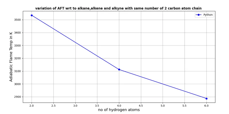
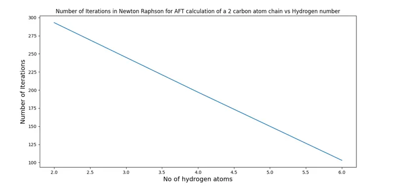
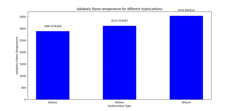
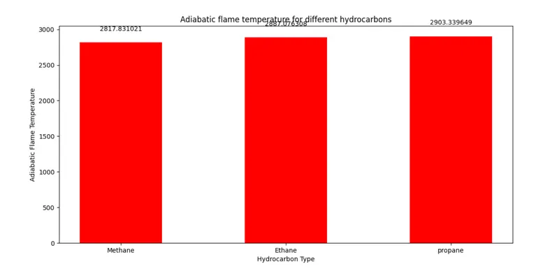
The above code consists of 3 cases. Case 1 deals with variation of AFT wrt to phi in constant volume chamber Case 2 deals with variation of AFT wrt to Alkane Alkene and Alkyne for a 2 carbon atom chain, Case 2 significantly represents the bond strength and Case 3 deals with variation of AFT wrt to different carbon atom chains (i.e Methane propane and Ethane )
steps :
- Consediring the Example of Methane for better understanding of the code
- CH4 + 2(O2+3.76N2) ---------> CO2 + 2H2O + 7.52 N2 (Stoichiometric case)
- Enthalpy H is a function of Temperature and Coefficients
- The coefficients are taken from NASA polynomial data which is chemkin II data
- After collecting the coefficients data the enthalpy is calculated in terms of Temperature
- H=(a1 + a2/2 T + a3/3 T^2 + a4/4 T^3 + a5/5 T^4 +a6/T) RT
- The NASA data file contains 14 coefficients for each and every species from which the first 7 represent high temperatute coefficents and last 7 represent low temperature coefficients, Depending on the local temperature ranges the co efficient data is taken
- Considering the gas to be ideal so the enthalpy is only the function of temperature
- Enthalpy of products and reactants are calculated in terms of temperature and use the equation dU = 0
- Now An polynomial equation is obtained in terms of Temperature which has to be solved for the T value which in turn gives the Adiabatic flame temperature value
- Newton Raphson method is used to solve for the T value
Case 1 : Variation of AFT wrt to Equivalence ratio
- Here hloss factor valued is fixed and a set of phi values are considered in order to examine how AFT is varied wrt to phi
- phi values are taken from 0.1 to 2 with interval of 0.1
- Newton Raphson solver code is run in a loop for different phi values and AFT is calculated at each phi value
- Later the same code is written by importing cantera and AFT is calculated at different phi values
case 2 and Case 3 :
a and b values are varied in the main code and the effect on AFT is observed . In Case 2 f function varies wrt to b and in Case 3 f function is variable wrt to T and an Alkane type is selected and code is written for 3 alkanes (C=1) Methane (C=2) Ethane and (C=3) propane with different functions seperately
Note : Case 2 and Case 3 in constant volume chamber can also be wriiten for constant pressure chamber.
Outputs :
Considering Ethane (i.e a=2 and b=6 and d=0)
Case 1 :
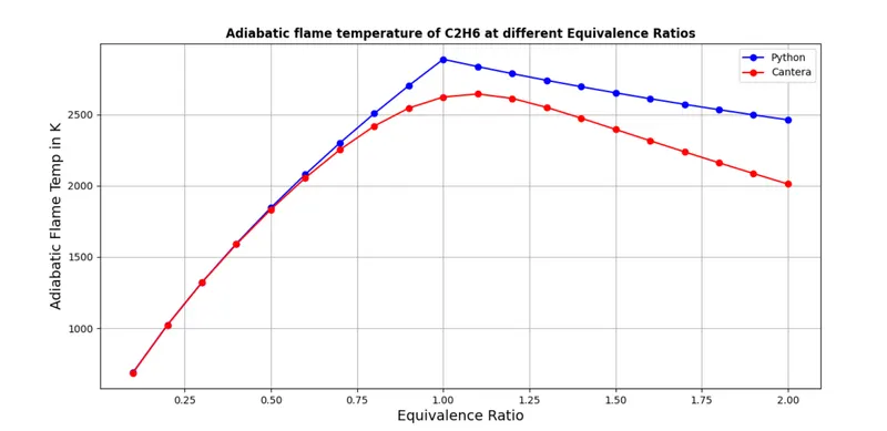
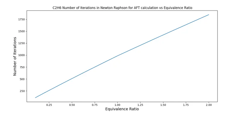
Case 2 :
Case 3:
Conclusion :
- Adiabatic flame temperature calculated in cantera code will be minimum when compared to python code because in python code all the products actually formed are not taken into account so some amount of heat will be utilized to increase the temperature of unconsidered products as cantera considers them its AFT calculation is accurate and lower
- With increase in phi value at first AFT increases and then it decreases due to improper combustion
- AFT in constant pressure will be lesser as compared to AFT in constant volume since some part of heat is used to perform work of expansion of volume to maintain the constant pressure
- If number of Carbon atoms are increased AFT also increases
- With increase in bond strength AFT also increases as more temperature is required to brake the bond so as a result AFT in Ethyne > Ethene > Ethane
References :
IC Engine combustion by SARA MCCALISTER