Writing a Program to solve Otto Cycle (Air Standard Cycle) & plotting PV Diagram using MATLAB

Main Code:

% Writing program to solve the otto cycle plotting the PV Diagram. 

% Otto cycle is the idealised thermodynamic cycle that describes the
% working of the spark ignition internal combustion engine. The otto cycle
% describes by PV diagram. The otto cycle completes its process in four
% stages.

% To connect all state points, we need to calculate piston kinematics
% equations. 
% Piston kinematics descibes how piston moves from the top dead centre to
% bottom dead centre and in this process how does combustion volume change
% with respect to crank angle.

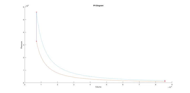
% Otto Cycle (Air Standard Cycle) stages in PV Diagram
% First stage is known as the isentropic compresssion stroke which means
% the process is frictionless, adiabatic & reversible. 
% The second stage is known as constant volume heat addition cycle.
% The third stage is isentropic expansion. 
% The fourth stage is the constant volume heat rejection process. 

% Following inputs has been given
% Engine geometric parameters which are bore = 0.1; stroke = 0.1;
% Connecting rod length (con_rod) = 0.15; Compressoion ratio (cr) = 12;
% Pressure at state 1 = 1 atmosphere = 101325 pa  & temperature = 500 k
% Specific Heat Ratio(gamma) = 1.4, temperature at state point 3 = 2300 k

close all
clear all
clc

% Inputs
gamma = 1.4; % Specific heat ration for air
t3 = 2300; % temperature at state 3 in kelvin

% state point 1
% State Variables at state point 1
p1 = 101325; % pressure in pascal(pa)
t1 = 500; % temperature unit - k

% Engine geometric parameters
bore = 0.1; % Cylinder bore dia in meter
stroke = 0.1; % % Engine stroke length in meter
con_rod = 0.15; % Connecting rod length in meter
cr = 12; % Compression Ratio

% Calculating the swept volume & the clearance volume
% Swept volume is the volume of cylinder
v_swept = (pi/4)*bore^2*stroke;
% clearance volume of cylinder
v_clearance = v_swept/(cr-1);

% Total volume
v1 = v_swept + v_clearance;
% Volume at TDC (Top Dead Centre)
v2 = v_clearance;

% State point 2
% As per Isentropic Compression process, p2v2^gamma = p1v1^gamma
% p2 = p1(v1/v2)^gamma = p1(cr)^gamma
p2 = p1*cr^gamma;

% Using Ideal gas law, p1v1/t1 = p2v2/t2 | t2 = p2v2t1/(p1v1)
t2 = p2*v2*t1/(p1*v1);

% To calculate compression volume
% As per Isentropic process, p1*v1^gamma = constant
constant_c = p1*v1^gamma;
% we are using 180 to 0 crank angle beacause its a compression state
v_compression = engine_kinematics(bore, stroke, con_rod, cr ,180,0);
% To calculate pressure during compression
p_compression = constant_c./v_compression.^gamma;


% state point 3
v3 = v2; % Volume remains constant between state 2-3

% Using Ideal gas law, p3v3/t3 = p2v2/t2 | p3 = p2t3/t2
p3 = p2*t3/t2;

% To calculate expansion volume
% As per Isentropic process, p3*v3^gamma = constant
constant_c = p3*v3^gamma;
% we are using 0 to 180 crank angle beacause its a expansion state
v_expansion = engine_kinematics(bore, stroke, con_rod, cr ,0, 180);
% To calculate pressure during compression
p_expansion = constant_c./v_expansion.^gamma;


% state point 4 
v4 = v1; % Volume remains constant between state 4-1

% As per Isentropic Compression process, 
% pev3^gamma = p4v4^gamma | p4 = p3(v3/v4)^gamma
p4 = p3*(v3/v4)^gamma;

% To determine the thermal efficiency of the cycle
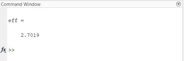
eff = 1 - (1 - (cr^(gamma -1)))

% Plotting 
figure(1)
hold on
plot(v1,p1, '*', 'color', 'r') % state point 1
plot(v_compression, p_compression) % Compression curve between 1 & 2
plot(v2,p2, '*', 'color', 'r') % state point 2
plot(v3,p3, '*', 'color', 'r') % state point 3
plot([v2 v3], [p2 p3], 'color','b') % Connecting state point 2 & 3
plot(v_expansion, p_expansion) % Expansion curve between 3 & 4
plot(v4,p4, '*', 'color', 'r') % state point 4
plot([v4 v1], [p4 p1], 'color','b') % Connecting state points 4 & 1

xlabel('Volume') % X-axis name
ylabel('Pressure') % Y-axis name
title('PV Diagram') % Plot title

Function code:

function [v] = engine_kinematics(bore, stroke, con_rod, cr, start_crank, end_crank)

% To determine how combustion volume changes inside the engine, following
% piston kinematics equation is used. Equation has been derived based on
% the geometric relationships.
% (v/v_c) = 1 + 0.5(cr-1)[R + 1 - cosd(theta) - (R^2 - sind(theta)^2)^0.5]


% Inputs
a = stroke/2; % Crank pin radius
R = con_rod/a; % Ratio

theta = linspace(start_crank,end_crank, 100); % Crank Angle in degree

% Calculating the swept volume & the clearance volume of cylinder
% Swept volume is the volume of cylinder
v_s = (pi/4)*bore^2*stroke;
% Clearance volume
v_c = v_s/(cr-1);

% Dividing the above mentioned piston kinematics equations into number of
% individual terms
term1 = 0.5*(cr-1);
term2 = R + 1 - cosd(theta);
term3 = (R^2 - sind(theta).^2).^0.5;

v = (1 + term1*(term2 - term3)).*v_c; % Volume

end

Results:

1) PV Diagram

2) Thermal Efficiency: