Writing A MATLAB/Octave Program Using Jacobi
Problem Statement:-
1. Steady-state analysis & Transient State Analysis
Solve the 2D heat conduction equation by using the point iterative techniques that were taught in the class. The Boundary conditions for the problem are as follows;
Top Boundary = 600 K
Bottom Boundary = 900 K
Left Boundary = 400 K
Right Boundary = 800 K
You will implement the following methods for solving implicit equations.
1. Jacobi
2. Gauss-seidel
3. Successive over-relaxation
Your absolute error criteria is 1e-4
Abstract:- The work is focused on writing several MATLAB/Octave codes to solve steady & unsteady (transient) state 2D heat conduction equations by using the point iterative techniques such as Jacobi, Gauss-seidel & Successive Over Relaxation (SOR) for both implicit & explicit schemes. The problem statement requires us to assume that the domain is a square i.e. the number of node points along the X-axis is equal to the Y-axis. The necessary Boundary Conditions are provided to us as:- Top Boundary = 600 K, Bottom Boundary = 900 K, Left Boundary = 400Ti,j=dy2⋅(Ti+1,j+Ti-1,j)+dx2⋅(Ti,j+1+Ti,j-1)2⋅(dx2+dy2)">K, Right Boundary = 800 K. This project has been divided into two parts. Part 1, focuses on solving the problem using a Steady-state solver & then comparing the results for Jacobi, Gauss-seidel & Successive Over Relaxation (SOR) schemes. While Part 2, deals with solving the problem using a transient solver using both Implicit & Explicit methods & then compares the results for Jacobi, Gauss-seidel & Successive Over Relaxation (SOR) schemes.
Theory:-
Part 1: Steady-State Analysis of the 2D heat conduction
`((∂^2T)/(∂x^2))+((∂^2T)/(∂y^2))=0`
Next, we apply the central differencing scheme to discretize the equation
`((∂^2T)/(∂x^2)) = (T_(i−1,j) − 2(T_(i,j)) + (T_(i+1,j)))/(Δx^2)`
`((∂^2T)/(∂y^2)) = (T_(i,j-1) − 2(T_(i,j)) + (T_(i,j+1)))/(Δy^2)`
Adding the two equations we get
`((∂^2T)/(∂x^2)) = (T_(i−1,j) − 2(T_(i,j)) + (T_(i+1,j)))/(Δx^2) + ((∂^2T)/(∂y^2)) = (T_(i,j-1) − 2(T_(i,j)) + (T_(i,j+1)))/(Δy^2) = 0`
we know Nx=Ny=nodes on each sides are equal,
we can consider `triangle x = triangle y`, on rearranging we get
`T i , j = 1 /4 ( T i − 1 , j + T i + 1 , j + T i , j − 1 + T i , j + 1 )`
MATLAB/Octave program code (Steady-state)
                                                    #Main Program code to solve the Steady-State 2D Heat Conduction problem
------------------------------------------------------------------------------------------------------------------------------------------------------------------
clear all
close all
clc

%inputs

nx = 10               % number of grid points along x axis
ny = nx ;             %since given domain is a square

x = linspace(0,1,nx);
dx = x(2)-x(1);
y = linspace(0,1,ny);
z = fliplr(y);
f = 1.5;
iter = 1;

t = ones([nx,ny])*298;

% Applying the given Boundary Conditions

t(1,1:nx) = 600;
t(ny,1:nx) = 900;
t(2:ny-1,1) = 400;
t(2:ny-1,nx) = 800;

% Creating a copy

told = t;
r1 = t;

error = 19;
tol = 1e-4;


for iterative_solver=1:3;
  while(error>tol);
  for i=2:nx-1;
    for j=2:ny-1;
      if(iterative_solver==1);
      t(i,j)=jacobi(t,told,i,j);
      elseif(iterative_solver==2)
      t(i,j)=GS(t,told,i,j);
    else
      t(i,j)=sor(t,told,i,j,f);
      end
      end
    end


 error = max(max(t-told));
        told = t;
        [u1,v1] = meshgrid(x,z);

%plotting the contours

if(iterative_solver==1);

figure (1);
contourf(u1,v1,t);
[C,h]=contourf(u1,v1,t);
colorbar;
colormap(jet);
clabel(C,h);
xlabel('x-axis');
ylabel('y-axis');
title_text=sprintf('jacobi iterantion number = %d',iter);
title(title_text);
pause(0.003);

elseif(iterative_solver==2);


figure (2);
contourf(u1,v1,t);
[C,h]=contourf(u1,v1,t);
colorbar;
colormap(jet);
clabel(C,h);
xlabel('x-axis');
ylabel('y-axis');
title_text=sprintf('GS iterantion number = %d',iter);
title(title_text);
pause(0.003);
else


figure (3);
[C,h]=contourf(u1,v1,t);
colorbar;
colormap(jet);
clabel(C,h);
xlabel('x-axis');
ylabel('y-axis');
title_text=sprintf('sor iterantion number = %d',iter);
title(title_text);
pause(0.003);
end


iter = iter+1;
end

error = 19;
iter = 1;
t = r1;
told = r1;

end
#User Defined Function (UDF) for Steady-State Jacobi scheme
-------------------------------------------------------------------------------------------------------------------------------------------------------------------------
function out = jacobi(t,told,i,j)
out=0.25*((told(i,j-1)+told(i,j+1)+told(i-1,j)+told(i+1,j)));
end #User Defined function(UDF) for Gauss-Seidal Scheme
------------------------------------------------------------------------------------------------------------------------------------------------------------------------------
function out = GS(t,told,i,j)
out=0.25*(t(i,j-1)+told(i,j+1)+t(i-1,j)+told(i+1,j));
end #User Defined Function (UDF) for Steady-State Successive Over Relaxation(SOR) scheme
--------------------------------------------------------------------------------------------------------------------------------------------------------------------------
function out = sor(t,told,i,j,f)
out =((1-f)*told(i,j)+(f*0.25*(t(i,j-1)+told(i,j+1)+t(i-1,j)+told(i+1,j))));
end
Observations & Conclusion (Steady-state) :-
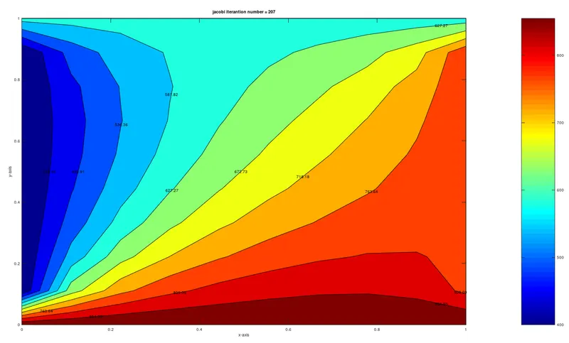
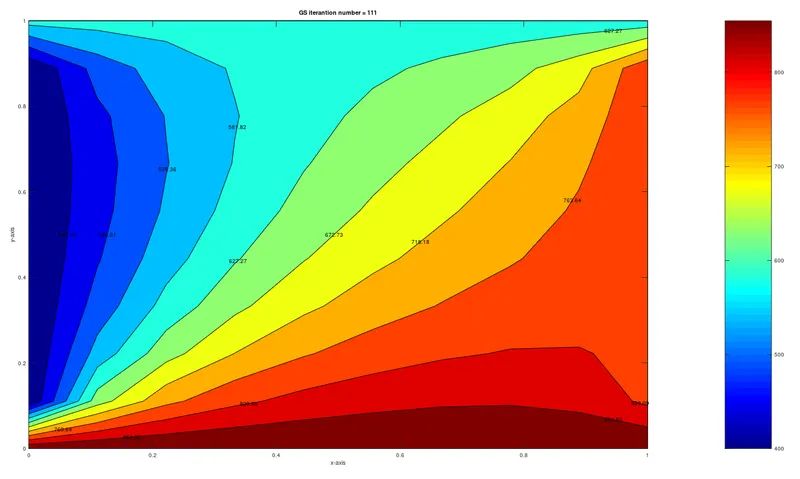
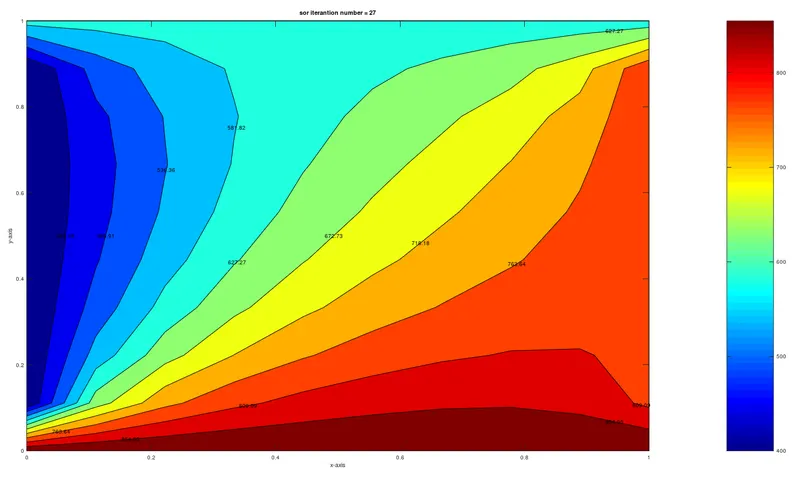
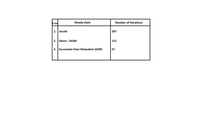
From the above three contour plots, we can conclude that for steady-state analysis of a 2D heat conduction problem the Successive Over Relaxation (SOR) Scheme requires much lower iterations to reach the desired solution than Gauss-Siedel & Jacobi schemes which took 111 & 207 iterations respectively. The number of iterations & stability of the solution depends on the relaxation factor for SOR. If the relaxation factor reaches a value of 0 then it will lead to under-relaxation which would then again increase the number of iterations, vice versa if the relaxation factor is high then it will lead to the solution to blow off.
Part 2: Unsteady/Transient State Analysis of the 2D heat conduction (Explicit & Implicit)
(i) Solving using Explicit Method
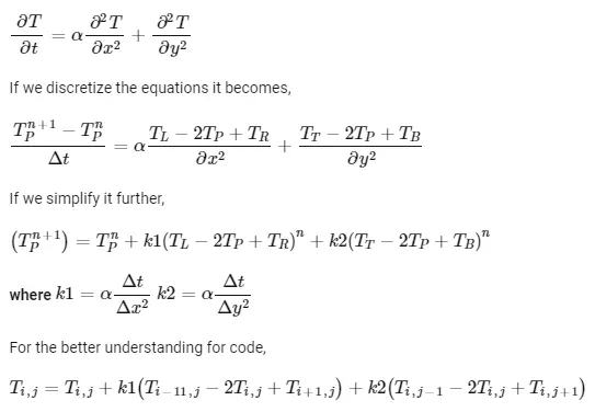
The 2-D heat equation for an unsteady/transient state is given by,
MATLAB/Octave program code (Transient-state, Explicit)
                                                      #Main Program code to solve the Transient/Unsteady state 2D Heat Conduction problem (Explicit Scheme)
---------------------------------------------------------------------------------------------------------------------------------------------------------------------


close all
clear all
clc

%Solving the Unsteady state 2D heat conduction (EXPLICIT SCHEME)

%Input Parameters
%Number of grid points
nx = 10;
ny = nx;
nt = 1400;

x = linspace(0,1,nx);
y = linspace(0,1,ny);

dx = x(2) - x(1);
dy = dx;

%Absolute error criteria > tolerance
error = 9e9;
tolerance = 1e-4;
dt = 1e-3;
omega = 1.1;

%Defining Boundary conditions
T_L = 400;
T_T = 600;
T_R = 800;
T_B = 900;

T = 300*ones(nx,ny);

T(2:ny - 1, 1)  = T_L;
T(2:ny - 1, nx) = T_R;
T(1, 2:nx - 1)  = T_T;
T(ny, 2:nx - 1) = T_B;

%Calculating Average temperature at corners
T(1,1) = (T_T + T_L)/2;
T(nx,ny) = (T_R + T_B)/2;
T(1,ny) = (T_T + T_R)/2;
T(nx,1) = (T_L + T_B)/2;

%Assigning orginal values to T
T_intial = T;
T_old = T;


%Calculation of 2D steady heat conduction EQUATION by Successive over-relaxation method
iterative_solver = 1;
k1 = 1.1*(dt/(dx^2));
k2 = 1.1*(dt/(dy^2));

if iterative_solver == 1
    Steady_Explicit = 1;
    for k = 1:nt
        error = 1;

        while(error > tolerance)

            for i = 2:nx - 1

                for j = 2:ny - 1
                    Term_1 = T_old(i,j);
                    Term_2 = k1*(T_old(i+1,j) - 2*T_old(i,j) + (T_old(i-1,j)));
                    Term_3 = k2*(T_old(i,j+1) - 2*T_old(i,j) + T_old(i,j-1));
                    T(i,j) = Term_1 + Term_2 + Term_3;
                end

            end

            error = max(max(abs(T_old - T)));
            T_old = T;
            Steady_Explicit = Steady_Explicit + 1;

        end
    end
end

%Plotting
figure(1)
contourf(x,y,T)
clabel(contourf(x,y,T))
colorbar
colormap(jet)
set(gca, 'ydir', 'reverse')

xlabel('X-Axis')
ylabel('Y-Axis')
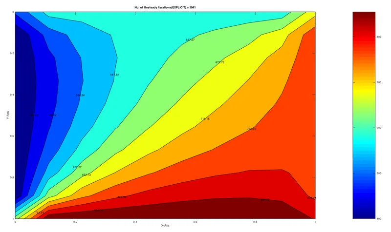
title(sprintf('No. of Unsteady Iterations(EXPLICIT) = %d', Steady_Explicit));
pause(0.03);
Results:-
(ii) Solving using Implicit Method
MATLAB/Octave program code for Jacobi Scheme (Transient-state, Implicit)
                                              #MATLAB/Octave code for solving Unsteady/Transient state 2D heat conduction by Jacobi Method (IMPLICIT SCHEME)
------------------------------------------------------------------------------------------------------------------------------------------------------------------------------

close all
clear all
clc


%Input Parameters
%Number of grid points
nx = 10;
ny = nx;
nt = 1400;

x = linspace(0,1,nx);
y = linspace(0,1,ny);

dx = x(2) - x(1);
dy = dx;

%Absolute error criteria > tolerance
error = 9e9;
tolerance = 1e-4;
dt = 1e-3;

%Defining Boundary conditions
T_L = 400;
T_T = 600;
T_R = 800;
T_B = 900;

T = 300*ones(nx,ny);

T(2:ny - 1, 1)  = T_L;
T(2:ny - 1, nx) = T_R;
T(1, 2:nx - 1)  = T_T;
T(ny, 2:nx - 1) = T_B;

%Calculating Average temperature at corners
T(1,1) = (T_T + T_L)/2;
T(nx,ny) = (T_R + T_B)/2;
T(1,ny) = (T_T + T_R)/2;
T(nx,1) = (T_L + T_B)/2;

%Assigning orginal values to T
T_old = T;
T_intial = T;

%Calculation of 2D steady heat conduction EQUATION by Successive over-relaxation method
k1 = 1.1*(dt/(dx^2));
k2 = 1.1*(dt/(dy^2));

Jacobi_iteration = 1;
for k = 1:nt
    error = 9e9;

    while(error > tolerance)

        for i = 2:nx - 1

            for j = 2:ny - 1

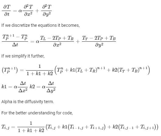
                Term_1 = 1/(1 + (2*k1) + (2*k2));
                Term_2 = k1*Term_1;
                Term_3 = k2*Term_1;
                H = (T_old(i-1,j)) + (T_old(i+1,j));
                V = (T_old(i,j+1)) + (T_old(i,j-1));

                T(i,j) = (T_intial(i,j)*Term_1) + (H*Term_2) + (V*Term_3);

            end

        end

        error = max(max(abs(T_old - T)));

        T_old = T;
        Jacobi_iteration = Jacobi_iteration + 1;

    end

    T_intial = T;

    %Plotting
    figure(1)
    contourf(x,y,T)
    clabel(contourf(x,y,T))
    colorbar
    colormap(jet)
    set(gca, 'ydir', 'reverse')

    xlabel('X-Axis')
    ylabel('Y-Axis')
    title(sprintf('No. of Unsteady Jacobi Iterations(IMPLICIT) = %d', Jacobi_iteration));
    pause(0.03)

end
MATLAB/Octave program code for Gauss-Siedel (Transient-state, Implicit)
                                              #MATLAB/Octave code for solving Unsteady/Transient state 2D heat conduction by Gauss-seidel Method (IMPLICIT SCHEME)
-----------------------------------------------------------------------------------------------------------------------------------------------------------------------

close all
clear all
clc


%Input Parameters
%Number of grid points
nx = 10;
ny = nx;
nt = 1400;

x = linspace(0,1,nx);
y = linspace(0,1,ny);

dx = x(2) - x(1);
dy = dx;

%Absolute error criteria > tolerance
error = 9e9;
tolerance = 1e-4;
dt = 1e-3;

%Defining Boundary conditions
T_L = 400;
T_T = 600;
T_R = 800;
T_B = 900;

T = 300*ones(nx,ny);

T(2:ny - 1, 1)  = T_L;
T(2:ny - 1, nx) = T_R;
T(1, 2:nx - 1)  = T_T;
T(ny, 2:nx - 1) = T_B;

%Calculating Average temperature at corners
T(1,1) = (T_T + T_L)/2;
T(nx,ny) = (T_R + T_B)/2;
T(1,ny) = (T_T + T_R)/2;
T(nx,1) = (T_L + T_B)/2;

%Assigning orginal values to T
T_old = T;
T_intial = T;

%Calculation of 2D steady heat conduction EQUATION by Successive over-relaxation method
k1 = 1.1*(dt/(dx^2));
k2 = 1.1*(dt/(dy^2));

Gauss_Seidel_iteration = 1;
for k = 1:nt
    error = 9e9;

    while(error > tolerance)

        for i = 2:nx - 1

            for j = 2:ny - 1

                Term_1 = 1/(1 + (2*k1) + (2*k2));
                Term_2 = k1*Term_1;
                Term_3 = k2*Term_1;
                H = (T(i-1,j)) + (T_old(i+1,j));
                V = (T(i,j+1)) + (T_old(i,j-1));

                T(i,j) = (T_intial(i,j)*Term_1) + (H*Term_2) + (V*Term_3);

            end

        end

        error = max(max(abs(T_old - T)));
        T_old = T;
        Gauss_Seidel_iteration = Gauss_Seidel_iteration + 1;

    end

    T_intial = T;

    %Plotting
    figure(1)
    contourf(x,y,T)
    clabel(contourf(x,y,T))
    colorbar
    colormap(jet)
    set(gca, 'ydir', 'reverse')

    xlabel('X-Axis')
    ylabel('Y-Axis')
    title(sprintf('No. of Unsteady Gauss-Seidel Iterations(IMPLICIT) = %d', Gauss_Seidel_iteration));
    pause(0.03)

end
MATLAB/Octave program code for SOR (Transient-state, Implicit)
                                                      #MATLAB/Octave code for solving Unsteady/Transient state 2D heat conduction by Successive over-relaxation Method (SOR)(IMPLICIT SCHEME)
----------------------------------------------------------------------------------------------------------------------------------------------------------------------------

close all
clear all
clc


%Input Parameters
%Number of grid points
nx = 10;
ny = nx;
nt = 1400;

x = linspace(0,1,nx);
y = linspace(0,1,ny);
dx = x(2) - x(1);


dy = dx;

%Absolute error criteria > tolerance
error = 9e9;
tolerance = 1e-4;
dt = 1e-3;
omega = 1.1;

%Defining Boundary conditions
T_L = 400;
T_T = 600;
T_R = 800;
T_B = 900;

T = 300*ones(nx,ny);

T(2:ny - 1, 1)  = T_L;
T(2:ny - 1, nx) = T_R;
T(1, 2:nx - 1)  = T_T;
T(ny, 2:nx - 1) = T_B;

%Calculating Average temperature at corners
T(1,1) = (T_T + T_L)/2;
T(nx,ny) = (T_R + T_B)/2;
T(1,ny) = (T_T + T_R)/2;
T(nx,1) = (T_L + T_B)/2;

%Assigning orginal values to T
T_old = T;
T_intial = T;
T_end = T;

%Calculation of 2D steady heat conduction EQUATION by Successive over-relaxation method
k1 = 1.1*(dt/(dx^2));
k2 = 1.1*(dt/(dy^2));

Successive_over_relaxation_iteration = 1;
for k = 1:nt
    error = 9e9;

    while(error > tolerance)

        for i = 2:nx - 1

            for j = 2:ny - 1

                Term_1 = 1/(1 + (2*k1) + (2*k2));
                Term_2 = k1*Term_1;
                Term_3 = k2*Term_1;
                H = (T(i-1,j)) + (T_old(i+1,j));
                V = (T(i,j+1)) + (T_old(i,j-1));

                T(i,j) = (T_intial(i,j)*Term_1) + (H*Term_2) + (V*Term_3);
                T_end(i,j) = ((1-omega)*T_old(i,j)) + (T(i,j)*omega);

            end

        end

        error = max(max(abs(T_old - T)));
        T_old = T_end;
        Successive_over_relaxation_iteration = Successive_over_relaxation_iteration + 1;

    end

    T_intial = T_end;

    %Plotting
    figure(1)
    contourf(x,y,T)
    clabel(contourf(x,y,T))
    colorbar
    colormap(jet)
    set(gca, 'ydir', 'reverse')

    xlabel('X-Axis')
    ylabel('Y-Axis')
    title(sprintf('No. of Unsteady SOR Iterations(IMPLICIT) = %d', Successive_over_relaxation_iteration));
    pause(0.03)

    end
Observations & conclusion:-
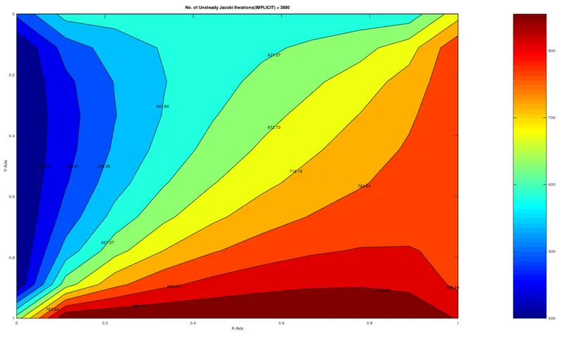
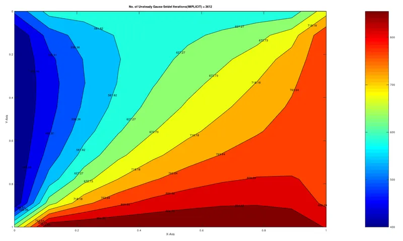
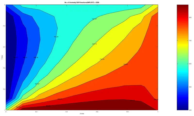
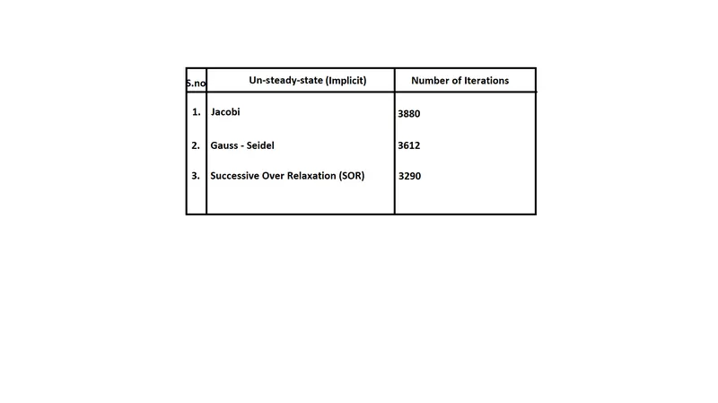
From the plots above we can observe that using a transient solver requires a larger number of iterations to converge than a steady-state solver. We can also notice that the Successive Over Relation (SOR) scheme takes a lower number of iterations to converge than Jacobi & Gauss-Siedel schemes. Therefore we can make a final conclusion that the steady-state solver yields quicker results & that the SOR technique is more effective for the 2D heat conduction problem as it can reach convergence sooner using both steady & transient solver.