Writing A MATLAB/Octave Code To Perform A 1D Super

Abstract:- The work is focused on writing a MATLAB/Octave code to simulate the isentropic flow through a quasi 1D supersonic nozzle using both the conservation and non-conservation forms of the governing equations and solving them using MacCormack's technique and compare their solutions by performing a grid dependency test. Through this project report, we will cover some important theory concepts such as: what is a nozzle? What is a supersonic flow & how do we define it inside a C-D nozzle? What is the MacCormack method & which governing equations we are using? The program will be divided into three parts, it will have the main program script followed by two separate user-defined functions (UDF) one for the conservative form & the other for the non-conservative form of the governing equation which will be called in the main MATLAB/Octave code.

Theory__________________________________________________________________________

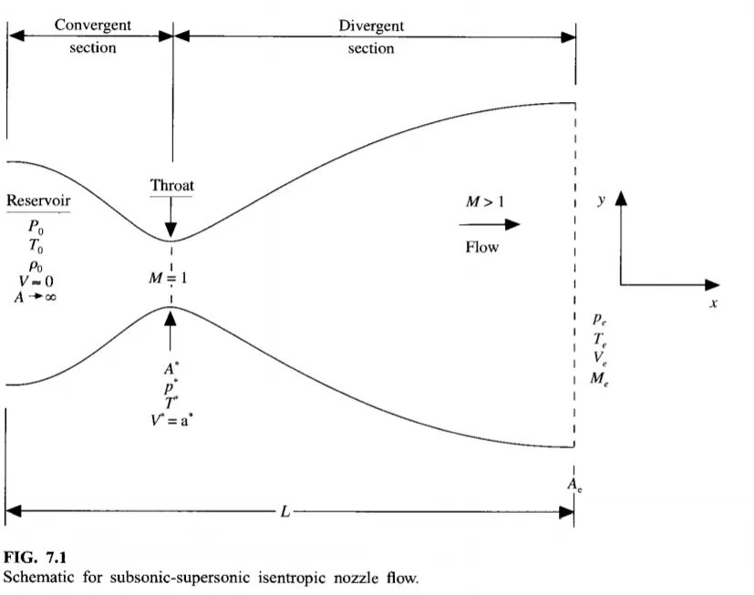
Ramjets, scramjets & rockets all use nozzles to accelerate hot exhaust to produce forward thrust as described by Newton's 3rd law of motion i.e. for every action there is an equal & opposite reaction. The amount of thrust produced by the engine depends on the mass flow rate (`dot{m} = frac {dm} {dt}` where = mass flow rate, = change in mass, = change in time) through the engine, the exit velocity of the flow, and the pressure at the exit of the engine. The value of these three flow variables are determined by the nozzle design. A nozzle is a relatively simple device, just a specially shaped tube through which hot gases flow. Ramjets and rockets typically use a fixed convergent section followed by a fixed divergent section for the design of the nozzle. This nozzle configuration is called a convergent-divergent, or CD, nozzle. In a CD nozzle, the hot exhaust leaves the combustion chamber and converges down to the minimum area, or throat, of the nozzle. The throat size is chosen to choke the flow and set the mass flow rate through the system. The flow in the throat is sonic which means the Mach number (M) is equal to one in the throat. Downstream of the throat, the geometry diverges and the flow is isentropically expanded to a supersonic Mach number that depends on the area ratio of the exit to the throat. The expansion of a supersonic flow causes the static pressure and temperature to decrease from the throat to the exit, so the amount of the expansion also determines the exit pressure and temperature. The exit temperature determines the exit speed of sound, which determines the exit velocity. The exit velocity, pressure, and mass flow through the nozzle determine the amount of thrust produced by the nozzle.

Conservation of Mass Equation:- `dotm = r * V * A =`constant, where `dotm`is the mass flow rate, r is the gas density, V is the gas velocity, and A is the cross-sectional flow area.

Conservation of Momentum Equation:- `r * V * dV = - dp`

Isentropic flow relation:- `((dp) / p) = gamma * (dr )/ r`, where `gamma` is defined as the ratio of specific heats [cp/cv] for air `gamma`= 1.4).

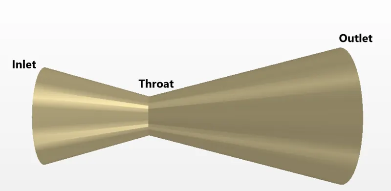
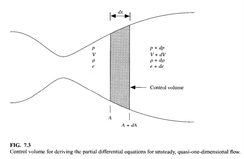
Quasi one dimensional implies that we still have variations of flow quantities in one direction only but we allow the cross-section area of stream tubes to vary along the same direction as well. This means that we will be able to analyze axisymmetric channels with varying cross-section areas such as convergent-divergent nozzles.

As gas is forced through a tube, the gas molecules are deflected by the walls of the tube. If the speed of the gas is much less than the speed of sound of the gas, the density of the gas remains constant and the velocity of the flow increases. However, as the speed of the flow approaches the speed of sound we must consider compressibility effects on the gas. The density of the gas varies from one location to the next. Considering flow through a tube, as shown in the figure, if the flow is very gradually compressed (area decreases) and then gradually expanded (area increases), the flow conditions return to their original values. We say that such a process is reversible. From a consideration of the second law of thermodynamics, a reversible flow maintains a constant value of entropy. Engineers call this type of flow an isentropic flow. Isentropic flows occur when the change in flow variables is small and gradual, such as the ideal flow through the nozzle shown above.

The ratio of the speed of the aircraft to the speed of sound in the gas determines the magnitude of many of the compressibility effects. Because of the importance of this speed ratio, aerodynamicists have designated it with a special parameter called the Mach number. The Mach number M allows us to define flight regimes in which compressibility effects vary.

`M = (Object speed)/(Speed of sound)`

1. Subsonic conditions occur for Mach numbers less than one, M < 1. For the lowest subsonic conditions, compressibility can be ignored.
2. As the speed of the object approaches the speed of sound, the flight Mach number is nearly equal to one, M = 1, and the flow is said to be transonic. At some places on the object, the local speed exceeds the speed of sound. Compressibility effects are most important in transonic flows and lead to the early belief in a sound barrier. Flight faster than sound was thought to be impossible. In fact, the sound barrier was only an increase in the drag near sonic conditions because of compressibility effects. Because of the high drag associated with compressibility effects, aircraft do not cruise near Mach 1.
3. Supersonic conditions occur for Mach numbers greater than one, 1 < M < 3. Compressibility effects are important for supersonic aircraft, and shock waves are generated by the surface of the object. For high supersonic speeds, 3 < M < 5, aerodynamic heating also becomes very important for aircraft design.
4. For speeds greater than five times the speed of sound, M > 5, the flow is said to be hypersonic. At these speeds, some of the energy of the object now goes into exciting the chemical bonds which hold together the nitrogen and oxygen molecules of the air. At hypersonic speeds, the chemistry of the air must be considered when determining forces on the object. The Space Shuttle re-enters the atmosphere at high hypersonic speeds, M ~ 25. Under these conditions, the heated air becomes an ionized plasma of gas and the spacecraft must be insulated from the high temperatures.

Non-Conservative form of the governing equations

Conservative form of the governing equations

In CFD, the MacCormack method is a widely used discretization scheme for the numerical solution of hyperbolic partial differential equations. MacCormack's method [1,2] is a predictor-corrector, finite-difference scheme that has been used for compressible flow and other applications for over twenty years. There exist both explicit and implicit versions of the algorithm, but the explicit predates the implicit by more than a decade, and it is considered one of the milestones of computational fluid dynamics. Both versions facilitate the solution of hyperbolic and parabolic equations by marching forward in time. The application of the MacCormack method is done in two steps; a predictor step which is followed by a corrector step. To illustrate the algorithm, consider the following first-order hyperbolic equation

Predictor step: In the predictor step, a "provisional" value of at time level (denoted by ) is estimated as follows

The above equation is obtained by replacing the spatial and temporal derivatives in the previous first-order hyperbolic equation using forward differences.

Corrector step: In the corrector step, the predicted value {displaystyle u_{i}^{overline {n+1}}} is corrected according to the equation

Note that the corrector step uses backward finite difference approximations for spatial derivative. The time-step used in the corrector step is in contrast to the used in the predictor step.

Replacing the term by the temporal average

to obtain the corrector step as

Apply Predictor Step to the Non-Conservative form of the governing equations

Find out time derivative at all the pints.

`(((∂ρ)/(∂t))^t)_i=−(ρ^t)_i[((V^t)_(i+1)−(V^t)_i)/(Δx)] − (ρ^t)_i(V^t)_i [(ln(A_(i+1)) − ln(A_i))/(Δx)] − (V^t)_i[((ρ^t)_(i+1)−(ρ^t)_i)/(Δx)]` `(((∂V)/(∂t))^t)_i = −(V^t)_i[((V^t)_(i+1)−(V^t)_i)/(Δx)] −1/γ [((T^t)_(i+1)−(T^t)_i)/(Δx) +((T^t)_i)/(ρ^t)_i(((ρ^t)_(i+1)−(ρ^t)_i)/(Δx))]` `(((∂T)/(∂x))^t)_i = (V^t)_i [((T^t)_(i+1)−(T^t)_i)/(Δx)] - (gamma-1)(T^t)_i[((V^t)_(i+1)−(V^t)_i)/(Δx) + (V^t)_i [(ln(A_(i+1)) − ln(A_i))/(Δx)]`

Apply Corrector Step to the Non-Conservative form of the governing equations

Find time derivative values at time (t+dt) with the predicted values.

`(((∂ρ)/(∂t))^(t+Δt))_i = −((¯ρ)^(t+Δt))_i [((V^(t+trianglet))_(i)−(V^(t+trianglet))_(i-1))/(Δx)] − (ρ^t)_i(V^(t+trianglet))_i [(ln(A_(i)) − ln(A_(i-1)))/(Δx)] − (V^(t+trianglet))_(i)[((ρ^(t+trianglet))_(i)−(ρ^(t+trianglet))_(i-1))/(Δx)]`

`(((∂V)/(∂t))^(t+trianglet))_i = −(V^(t+trianglet))_i [((V^(t+trianglet))_(i+1)−(V^(t+trianglet))_(i-1))/(Δx)] −1/γ [((T^(t+trianglet))_(i)−(T^(t+trianglet))_(i-1))/(Δx) +((T^(t+trianglet))_i)/(ρ^(t+trianglet))_i(((ρ^(t+trianglet))_(i)−(ρ^(t+trianglet))_(i-1))/(Δx))]`

`(((∂T)/(∂x))^(t+trianglet))_i = (V^(t+trianglet))_i [((T^(t+trianglet))_(i)−(T^(t+trianglet))_(i-1))/(Δx)] - (gamma-1)(T^(t+trianglet))_i[((V^(t+trianglet))_(i)−(V^(t+trianglet))_(i-1))/(Δx) + (V^(t+trianglet))_i [(ln(A_(i)) − ln(A_(i-1)))/(Δx)]`

Similarly, we compute the Predictor Step & Corrector Step to the Conservative form of the governing equations as well.

Main MATLAB/Octave Script________________________________________________

                                          %Writing a MATLAB/Octave Program Code To Solve The Quasi 1D Supersonic Nozzle Flow Equations  
----------------------------------------------------------------------------------------------------------------------------------------------------------------


clear all
close all
clc

%INPUT PARAMETERS   
n = 31;             
gamma = 1.4;
x = linspace(0,3,n);
dx = x(2) - x(1);

%No. of time step
nt = 1400;

%Courant Number
C = 0.5;            


%FUNCTION FOR NON CONSERVATIVE FORM

tic;
[Mass_flow_rate_NC, Pressure_NC, Mach_number_NC, rho_NC, v_NC, T_NC, rho_throat_NC, v_throat_NC, T_throat_NC, Mass_flow_rate_throat_NC, Pressure_throat_NC, Mach_number_throat_NC] = Non_conservative_form(x, dx, n, gamma, nt, C);
Time_elapsed_NC = toc;
fprintf('Time Elasped for Non Conservative form: %0.4f', Time_elapsed_NC);
hold on

%PLOTTING 
%Timestep variation of properties at throat area in Non Conservative form
figure(2)

%Density
subplot(4,1,1)
plot(linspace(1,nt,nt),rho_throat_NC,'color','m')
ylabel('Density')
legend({'Density at throat'});
axis([0 1400 0 1.3]);
grid minor;
title('Timestep variation at throat area - NON CONSERVATIVE FORM')

%Temperature
subplot(4,1,2)
plot(linspace(1,nt,nt),T_throat_NC,'color','c')
ylabel('Temperature')
legend({'Temperature at throat'});
axis([0 1400 0.6 1]);
grid minor;

%Pressure
subplot(4,1,3)
plot(linspace(1,nt,nt),Pressure_throat_NC,'color','g')
ylabel('Pressure')
legend({'Pressure at throat'});
axis([0 1400 0.4 1.1]);
grid minor

%Mach Number
subplot(4,1,4)
plot(linspace(1,nt,nt),Mach_number_throat_NC,'color','y')
xlabel('Timesteps')
ylabel('Mach Number')
legend({'Mach Number at throat'});
axis([0 1400 0.6 1.4]);
grid minor;


%Steady state simulation for primitve values for Non Conservative form
figure(3);
%Density

subplot(4,1,1);
plot(x,rho_NC,'color','m')
ylabel('Density')
legend({'Density'});
axis([0 3 0 1])
grid minor;
title('Variation of Flow Rate Distribution - NON CONSERVATIVE')

%Temperature
subplot(4,1,2);
plot(x,T_NC,'color','c')
ylabel('Temperature')
legend({'Temperature'});
axis([0 3 0 1])
grid minor;

%Pressure
subplot(4,1,3);
plot(x,Pressure_NC,'color','g')
ylabel('Pressure')
legend({'Pressure'});
axis([0 3 0 1])
grid minor;

%Mach number
subplot(4,1,4);
plot(x,Mach_number_NC,'color','y')
xlabel('Nozzle Length')
ylabel('Mach number')
legend({'Mach number'});
axis([0 3 0 4])
grid minor;


%FUNCTION FOR CONSERVATIVE FORM
tic;
[Mass_flow_rate_C, Pressure_C, Mach_number_C, rho_C, v_C, T_C, rho_throat_C, v_throat_C, T_throat_C, Mass_flow_rate_throat_C, Pressure_throat_C, Mach_number_throat_C] = Conservative_form(x, dx, n, gamma, nt, C);
Time_elasped_C = toc;
fprintf('Time Elasped for Conservative form: %0.4f', Time_elasped_C);

%PLOTTING 
%Timestep variation of properties at throat area in Conservative form
figure(5)

%Density
subplot(4,1,1)
plot(rho_throat_C,'color','m')
ylabel('Density')
legend({'Density at throat'});
axis([0 1400 0 1]);
grid minor;
title('Timestep variation at throat area - CONSERVATIVE FORM')

%Temperature
subplot(4,1,2)
plot(T_throat_C,'color','c')
ylabel('Temperature')
legend({'Temperature at throat'});
axis([0 1400 0.6 1]);
grid minor;

%Pressure
subplot(4,1,3)
plot(Pressure_throat_C,'color','g')
ylabel('Pressure')
legend({'Pressure at throat'});
axis([0 1400 0.2 0.8]);
grid minor

%Mach Number
subplot(4,1,4)
plot(Mach_number_throat_C,'color','y')
xlabel('Timesteps')
ylabel('Mach Number')
legend({'Mach Number at throat'});
axis([0 1400 0.6 1.4]);
grid minor;


%Steady state simulation for primitve values for Non Conservative form
figure(6);

%Density 
subplot(4,1,1);
plot(x,rho_C,'color','m')
ylabel('Density')
legend({'Density'});
axis([0 3 0 1])
grid minor;
title('Variation of Flow Rate Distribution - CONSERVATIVE FORM')

%Temperature 
subplot(4,1,2);
plot(x,T_C,'color','c')
ylabel('Temperature')
legend({'Temperature'});
axis([0 3 0 1])
grid minor;

%Pressure
subplot(4,1,3);
plot(x,Pressure_C,'color','g')
ylabel('Pressure')
legend({'Pressure'});
axis([0 3 0 1])
grid minor;

%Mach number
subplot(4,1,4);
plot(x,Mach_number_C,'color','y')
xlabel('Nozzle Length')
ylabel('Mach number')
legend({'Mach number'});
axis([0 3 0 4])
grid minor;


%COMPARISON PLOT of Normalized Mass Flow Rate of both forms
figure(7)
hold on
plot(x,Mass_flow_rate_NC,'r','linewidth',1.25)
hold on;
plot(x,Mass_flow_rate_C,'b','linewidth',1.25)
hold on;
grid on

legend('Non Conservative','Conservative'); %compare
xlabel('Length of the Domain')
ylabel('Mass Flow Rate')
title('Comparison of Normalized Mass Flow Rate of both forms')

Explanation For The Above Program (Main Script):

• Code starts with "clear all, close all and clc" which enables fresh start of a new program without the manipulation of previous values.
• Input parameters are assigned for the variables x, dx, n, gamma, nt, and C.
• Non-Conservative and Conservative forms are created as separate functions with the necessary inputs (User Defined Functions are attached below).
• The "tic toc" command was used for calculating the time elapsed between the functions.
• Plotting is done for the following solutions
  1)Timestep variation at throat area of both forms
  2)Variation of Flow Rate Distribution of both forms
  3)Comparison of Normalized Mass Flow Rate of both forms
• Each plot is computed as subplots of four primitive variables such as Density, Temperature, Pressure, and Mach Number at the throat of the Nozzle & as well as at the Convergent/Divergent section.

User Defined Function (UDF)________________________________________________

                                %Writting A User Defined Function(UDF) For Conservation Form of The Governing Equation
------------------------------------------------------------------------------------------------------------------------------------------------------------------------------

function [Mass_flow_rate_C, Pressure_C, Mach_number_C,  rho_C, v_C, T_C, rho_throat_C, v_throat_C, T_throat_C, Mass_flow_rate_throat_C, Pressure_throat_C, Mach_number_throat_C] = Conservative_form(x, dx, n, gamma, nt, C)

%Determining Initial profile of Density and Temperature
for i = 1:n
    
    if (x(i) >= 0 && x(i) <= 0.5)
        rho_C(i) = 1;
        T_C(i) = 1;
    elseif (x(i) >= 0.5 && x(i) <= 1.5)
        rho_C(i) = 1 - 0.366*(x(i) - 0.5);
        T_C(i) = 1 - 0.167*(x(i) - 0.5);
    elseif (x(i) >= 1.5 && x(i) <= 3)
        rho_C(i) = 0.634 - 0.3879*(x(i) - 1.5);
        T_C(i) = 0.833 - 0.3507*(x(i) - 1.5);
    end
    
end

%Area & Throat profiles
a = 1 + 2.2*(x - 1.5).^2;
throat = find(a==1);

%Initial profile fot Velocity and Pressure
v_C = 0.59./(rho_C.*a);
Pressure_C = rho_C.*T_C;

%Calculate the Initial Solution Vectors(U)
U1 = rho_C.*a;
U2 = rho_C.*a.*v_C;
U3 = rho_C.*a.*(T_C./(gamma - 1)) + ((gamma/2).*v_C.^2);


%Outer Time Loop
for k =1:nt
    
    %Time-step control
    dt = min(C.*dx./(sqrt(T_C) + v_C));
    
    %Saving a copy of Old Values
    U1_old = U1;
    U2_old = U2;
    U3_old = U3;

    %Calculating the Flux vector(F)
    F1 = U2;
    F2 = ((U2.^2)./U1) + ((gamma - 1)/gamma)*(U3 - (gamma/2)*((U2.^2)./U1));
    F3 = ((gamma*U2.*U3)./U1) - (gamma*(gamma - 1)*((U2.^3)./(2*U1.^2)));
    
    
    %Predictor Method
    for j = 2:n-1
    
        %Calculating the Source term(J)
        J2(j) = (1/gamma)*rho_C(j)*T_C(j)*((a(j + 1) - a(j))/dx);
        
        
        %Continuity Equation
        dU1_dt_P(j) = -((F1(j + 1) - F1(j))/dx);
        
        %Momentum Equation
        dU2_dt_P(j) = -((F2(j + 1) - F2(j))/dx) + J2(j);
        
        %Energy Equation
        dU3_dt_P(j) = -((F3(j + 1) - F3(j))/dx);
        
        
        %Updating New values
        U1(j) = U1(j) + dU1_dt_P(j)*dt;
        U2(j) = U2(j) + dU2_dt_P(j)*dt;
        U3(j) = U3(j) + dU3_dt_P(j)*dt;
        
    end
    
    %Updating Flux vectors
    F1 = U2;
    F2 = ((U2.^2)./U1) + ((gamma - 1)/gamma)*(U3 - ((gamma*0.5*(U2.^2))./(U1)));
    F3 = ((gamma*U2.*U3)./U1) - ((gamma*0.5*(gamma - 1)*(U2.^3))./(U1.^2));

    
    %Corrector Method
    for j = 2:n-1
        
        %Updating the Source term(J)
        J2(j) = (1/gamma)*rho_C(j)*T_C(j)*((a(j) - a(j - 1))/dx);

        %Simplifying the Equation's spatial terms
        dU1_dt_C(j) = -((F1(j) - F1(j - 1))/dx);
        dU2_dt_C(j) = -((F2(j) - F2(j - 1))/dx) + J2(j);
        dU3_dt_C(j) = -((F3(j) - F3(j - 1))/dx);

    end

    %Compute Average Time derivative
    dU1_dt = 0.5*(dU1_dt_P + dU1_dt_C);
    dU2_dt = 0.5*(dU2_dt_P + dU2_dt_C);
    dU3_dt = 0.5*(dU3_dt_P + dU3_dt_C);

    %Final Solution Update
    for i = 2:n-1
        U1(i) = U1_old(i) + dU1_dt(i)*dt;
        U2(i) = U2_old(i) + dU2_dt(i)*dt;
        U3(i) = U3_old(i) + dU3_dt(i)*dt;
        
    end
    
    
    %Applying Boundary Conditions
    %At Inlet
    U1(1) = rho_C(1)*a(1);
    U2(1) = 2*U2(2) - U2(3);
    
    v_C(1) = U2(1)./U1(1);
    U3(1) = U1(1)*((T_C(1)/(gamma - 1)) + ((gamma/2)*(v_C(1)).^2));
    
    %At Outlet
    U1(n) = 2*U1(n - 1) - U1(n - 2);
    U2(n) = 2*U2(n - 1) - U2(n - 2);
    U3(n) = 2*U3(n - 1) - U3(n - 2);
    
    %Final Primitive value update
    rho_C = U1./a;
    v_C = U2./U1;
    T_C = (gamma - 1)*((U3./U1 - (gamma/2)*(v_C).^2));
    
    %Defining Mass flow rate, Pressure and Mach number
    Mass_flow_rate_C = rho_C.*a.*v_C;
    Pressure_C = rho_C.*T_C;
    Mach_number_C = (v_C./sqrt(T_C));
    
    %Calculating Variables at throat section
    rho_throat_C(k) = rho_C(throat);
    T_throat_C(k) = T_C(throat);
    v_throat_C(k) = v_C(throat);
    Mass_flow_rate_throat_C(k) = Mass_flow_rate_C(throat);
    Pressure_throat_C(k) = Pressure_C(throat);
    Mach_number_throat_C(k) = Mach_number_C(throat);

    %PLOTTING
    %Comparison of non-dimensional Mass flow rates at different time steps
    figure(4)
    if k == 50
       plot(x, Mass_flow_rate_C, 'm', 'linewidth', 1.25);
       hold on
    elseif k == 100
       plot(x, Mass_flow_rate_C, 'c', 'linewidth', 1.25);
       hold on
    elseif k == 200
       plot(x, Mass_flow_rate_C, 'g', 'linewidth', 1.25);
       hold on
    elseif k == 400
       plot(x, Mass_flow_rate_C, 'y', 'linewidth', 1.25);
       hold on
    elseif k == 800
       plot(x, Mass_flow_rate_C, 'k', 'linewidth', 1.25);
       hold on
    end
           
    
    %Labelling
    title('Mass flow rates at different Timesteps - CONSERVATIVE FORM')
    xlabel('Distance')
    ylabel('Mass flow rate')
    legend({'50^t^h Timestep','100^t^h Timestep','200^t^h Timestep','400^t^h Timestep','800^t^h Timestep'})
    axis([0 3 0.4 1])
    grid on
    
end

end
  

Explanation of The UDF (Conservative form):

• The purpose of the function is to calculate the values of
  Mass flow rate, Pressure, Mach number, Density, velocity, Temperature, Density at the throat, the velocity at the throat, Temperature at the throat, Mass flow rate at the throat, Pressure at the throat, Mach number at the throat by the known equations for all the grid points (n=31).
  To determine the initial profile of Density & Temperature, for loop is used inputting the known conditions within an else-if command.
• Initial values of area, throat, velocity & Pressure are calculated using formulas.
• In order to simplify and avoid errors, the equation is split into Solution Vector(U), Flux Vector(F), and Source Term(J).
• Now Outer Time loop is computed for the loop to calculate all the grid points for various formulas inside the loop.
• MacCormack technique is used to solve the numerical solution of governing equations such as Continuity, Momentum & Energy Equation.
• The technique implies two methods for solving namely the Predictor method followed by the Corrector method.
• Predictor & Corrector methods are assigned within the for loop individually for calculating values.
• The calculated values are averaged in the next step and updating the solution with old values.
• Boundary Conditions are applied within the for loop and subsequently used for calculating the Mass Flow Rate, Mach Number & Pressure and also calculating the values throat section.
• Finally plotting is done for Distance(x) & Mass Flow Rate for different Timesteps.
• The program is ended.

                                      %Writting A User Defined Function (UDF) For Non-conservative Form of The Governing Equation
------------------------------------------------------------------------------------------------------------------------------------------------------------------------------

function [Mass_flow_rate_NC, Pressure_NC, Mach_number_NC, rho_NC, v_NC, T_NC, rho_throat_NC, v_throat_NC, T_throat_NC, Mass_flow_rate_throat_NC, Pressure_throat_NC, Mach_number_throat_NC] = Non_conservative_form(x, dx, n, gamma, nt, C)

%Intial boundary conditions
rho_NC = 1 - 0.3146*x;
T_NC = 1 - 0.2341*x;
v_NC = (0.1 + 1.09*x).*T_NC.^0.5;

%Area & Throat profiles
a = 1 + 2.2*(x - 1.5).^2;
throat = find(a==1);


%Outer Time Loop
for k = 1:nt
    
    %Time-step control
    dt = min(C.*dx./(sqrt(T_NC) + v_NC));
    
    %Saving a copy of Old Values
    rho_old = rho_NC;
    T_old = T_NC;
    v_old = v_NC;
    

    %Predictor Method
    for j = 2:n-1
        
        %Simplifying the Equation's spatial terms
        dv_dx = (v_NC(j + 1) - v_NC(j))/dx;
        drho_dx = (rho_NC(j + 1) - rho_NC(j))/dx;
        dT_dx = (T_NC(j + 1) - T_NC(j))/dx;
        dlog_a_dx = (log(a(j + 1)) - log(a(j)))/dx;
        
        %Continuity Equation
        drho_dt_P(j) = -rho_NC(j)*dv_dx - rho_NC(j)*v_NC(j)*dlog_a_dx - v_NC(j)*drho_dx;
        
        %Momentum Equation
        dv_dt_P(j) = -v_NC(j)*dv_dx - (1/gamma)*(dT_dx + (T_NC(j)*drho_dx/rho_NC(j)));
        
        %Energy Equation
        dT_dt_P(j) = -v_NC(j)*dT_dx - (gamma - 1)*T_NC(j)*(dv_dx + v_NC(j)*dlog_a_dx);
        
        
        %Solution Update
        rho_NC(j) = rho_NC(j) + drho_dt_P(j)*dt;
        v_NC(j) = v_NC(j) + dv_dt_P(j)*dt;
        T_NC(j) = T_NC(j) + dT_dt_P(j)*dt;
        
    end
    
    
    %Corrector Method
    for j = 2:n-1
        
        %Simplifying the Equation's spatial terms
        dv_dx = (v_NC(j) - v_NC(j - 1))/dx;
        drho_dx = (rho_NC(j) - rho_NC(j - 1))/dx;
        dT_dx = (T_NC(j) - T_NC(j - 1))/dx;
        dlog_a_dx = (log(a(j)) - log(a(j - 1)))/dx;
        
        %Continuity Equation
        drho_dt_C(j) = - rho_NC(j)*dv_dx - rho_NC(j)*v_NC(j)*dlog_a_dx - v_NC(j)*drho_dx;
        
        %Momentum Equation
        dv_dt_C(j) = - v_NC(j)*dv_dx - (1/gamma)*(dT_dx + (T_NC(j)*drho_dx/rho_NC(j)));
        
        %Energy Equation
        dT_dt_C(j) = - v_NC(j)*dT_dx - (gamma - 1)*T_NC(j)*(dv_dx + v_NC(j)*dlog_a_dx);
       
    end
    
    %Compute Average Time derivative
    drho_dt = 0.5.*(drho_dt_P + drho_dt_C);
    dv_dt = 0.5.*(dv_dt_P + dv_dt_C);
    dT_dt = 0.5.*(dT_dt_P + dT_dt_C);
    
    %Final Solution Update
    for i = 2:n-1
        rho_NC(i) = rho_old(i) + drho_dt(i)*dt;
        v_NC(i) = v_old(i) + dv_dt(i)*dt;
        T_NC(i) = T_old(i) + dT_dt(i)*dt;
        
    end
    
    %Applying Boundary Conditions
    %At Inlet
    rho_NC(1) = 1;
    v_NC(1) = 2*v_NC(2) - v_NC(3);
    T_NC(1) = 1;
    
    %At Outlet
    rho_NC(n) = 2*rho_NC(n-1) - rho_NC(n - 2);
    v_NC(n) = 2*v_NC(n - 1) - v_NC(n - 2);
    T_NC(n) = 2*T_NC(n - 1) - T_NC(n - 2);
    
    
    %Defining Mass flow rate, Pressure and Mach number
    Mass_flow_rate_NC = rho_NC.*a.*v_NC;
    Pressure_NC = rho_NC.*T_NC;
    Mach_number_NC = (v_NC./sqrt(T_NC));
    
    %Calculating Variables at throat section
    rho_throat_NC(k) = rho_NC(throat);
    T_throat_NC(k) = T_NC(throat);
    v_throat_NC(k) = v_NC(throat);
    Mass_flow_rate_throat_NC(k) = Mass_flow_rate_NC(throat);
    Pressure_throat_NC(k) = Pressure_NC(throat);
    Mach_number_throat_NC(k) = Mach_number_NC(throat);
    
    
    %PLOTTING
    %Comparison of non-dimensional Mass flow rates at different time steps
    figure(1);
    if k == 50
       plot(x, Mass_flow_rate_NC, 'm', 'linewidth', 1.25);
       hold on
    elseif k == 100
       plot(x, Mass_flow_rate_NC, 'c', 'linewidth', 1.25);
       hold on
    elseif k == 200
       plot(x, Mass_flow_rate_NC, 'g', 'linewidth', 1.25);
       hold on
    elseif k == 400
       plot(x, Mass_flow_rate_NC, 'y', 'linewidth', 1.25);
       hold on
    elseif k == 800
       plot(x, Mass_flow_rate_NC, 'k', 'linewidth', 1.25);
       hold on
    end
    
    %Labelling
    title('Mass flow rates at different Timesteps - NON CONSERVATIVE FORM)')
    xlabel('Distance')
    ylabel('Mass flow rate')
    legend({'50^t^h Timestep','100^t^h Timestep','200^t^h Timestep','400^t^h Timestep','800^t^h Timestep'})
    axis([0 3 0 2])
    grid on
    
end

end

Explanation of The UDF (Non-conservative form):

• The purpose of the function is to calculate the values of
  Mass flow rate, Pressure, Mach number, Density, velocity, Temperature, Density at the throat, the velocity at the throat, Temperature at the throat, Mass flow rate at the throat, Pressure at the throat, Mach number at the throat by the known equations for all the grid points.
• For this initial boundary conditions are established for Density, Temperature & Velocity, and profiles for calculating area & throat.
• Now Outer Time loop is computed for the loop to calculate all the grid points for various formulas inside the loop.
• MacCormack technique is used to solve the numerical solution of governing equations such as Continuity, Momentum & Energy Equation.
• The technique implies two methods for solving namely the Predictor method followed by the Corrector method.
• Predictor & Corrector methods are assigned within the for loop individually for calculating values.
• The calculated values are averaged in the next step and updating the solution with old values.
• Boundary Conditions are applied within the for loop and subsequently used for calculating the Mass Flow Rate, Mach Number & Pressure and also calculating the values throat section.
• Finally plotting is done for Distance(x) & Mass Flow Rate for different Timesteps.
• The program is ended.

Observation & Conclusion ________________________________________________

A. Plots For Time Step Variable At The Throat For Both Conservative & Non-conservative Form of Governing Equations

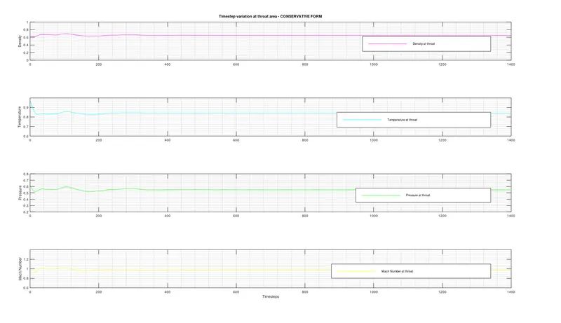
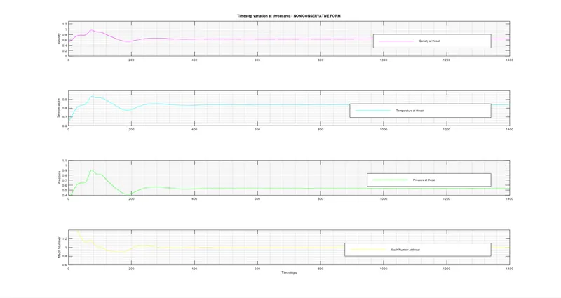
From the above plots, we can observe that the solution reaches a stable condition at around 200 iterations for the Conservative form while it takes 400 iterations for the Non-conservative form for the same grid points. For the Non-conservative form of Governing Equations, we observe few deviations during the initial phases which lead to a longer time to reach convergence. Therefore, we can conclude that the conservative form of the governing equation gives quicker results than that of the non-conservative form of the governing equation.

B. Plots For Variation For Flow Rate Distribution For Both Conservative & Non-conservative Form of Governing Equations

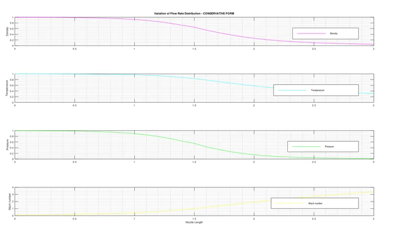
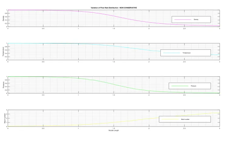
From the above plots, we can observe that for both conservative & non-conservative forms of the governing equations the flow rate distribution of Density, Temperature, Pressure & the Mach number is quite similar.

C. Plots For Mass Flow Rates At Different Time Steps For Both Conservative & Non-conservative Form of Governing Equations

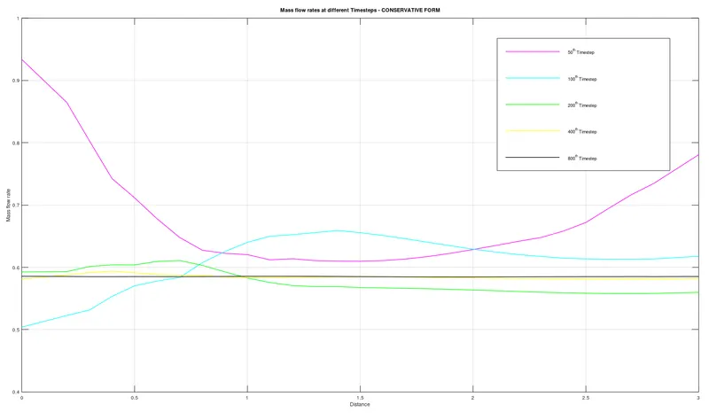
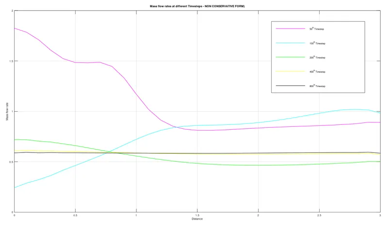
From the above plots, we can observe that the mass flow rate at the outlet for different time steps. Initially, the plots oscillate & remain unstable till the 200th timestep & then beacem stable & reached convergence for both Conservative & Non-conservative Form of Governing Equations.

D. Plot For Comparing Mass Flow Rate For Both Conservative & Non-conservative Form of Governing Equations

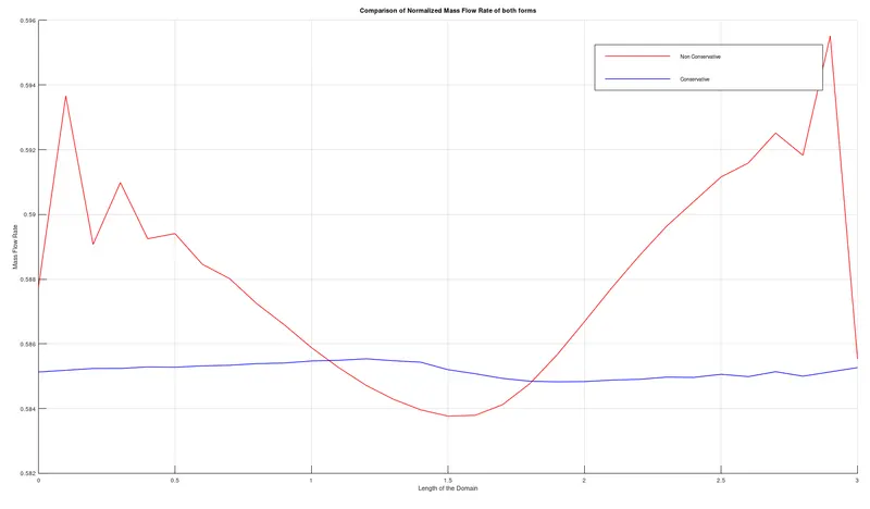
From the above plot, we can conclude that the Conservative form of the governing equation attains stability in a lesser number of iterations than the Non-conservative form of the governing equation.

Grid dependency is an important factor where we try to improve the solution by improving the mesh quality (adding more cells), so for our case, we increased the total number of grid points(n) from 31 to 61 and populated them in a sheet & run the case again. Upon running the simulation it was observed that the values are similar to the Primitive Variables for both the forms even when the Grid points(n) is changed from 31 to 61 showcasing that it doesn't get affected by the increase of grid points. Hence, we can conclude that the solution is grid-independent.