Writing A MATLAB/Octave Code To Analyze The Effect of Number of Grid Points On A Linear Convection Problem

Problem Statement:-

Numerical solution to the One-dimensional Linear Convection equation.

1. Assume that the domain length is L = 1m

2. The initial velocity profile is a step function. It is equal to 2m/s between x= 0.1 and 0.3 and 1m/s everywhere else

3. Use first-order forward differencing for the time derivative

4. Use first-order backward/rearward differencing for the space term.

5. Constant convection coefficient, c = 1 m/s

6. Time step, dt = 0.01

7. Simulation run time, t = 0.4 seconds.

Perform the simulation for the Number of nodes, n=20,40,80, and 160.

Objective:- The work is focused on solving the below-mentioned 1D Linear Convection equation using Finite Difference Method (FDM) where we will be making use of Forward Differencing (FD) scheme for the time derivative term & Backward Differencing (BD) scheme for the space term. The initial & final velocities are compared with various values of the number of divisions of the domain, denoted by 'n'. The goal is to plot these variations of 'n' for values of 20, 40, 80 & 160.

`(delu)/(delt) + C (delu)/(delx)`

where `(delu)/(delt)`= time derivative ; `(delu)/(delx)`= space term

Discretizing:-

We have the differential equation, `(delu)/(delt) + C (delu)/(delx)`

Applying Forward Difference scheme to the "time term" we get, `(delu)/(delt) = [u^(n+1)(i) - u^(n)(i)]/[trianglet]`

where, `(delu)/(dt)`= First Order time derivative of velocity

`u^(n+1)(i) =` Velocity at node (i) & time step (n+1)

`u^(n)(i)=` velocity at node (i) at time step (n)

`triangle t = time step`

Applying Backward Difference scheme to the "time term" we get `(delu)/(delx) = [u^(n)(i) - u^(n)(i-1)]/(trianglex)`

where, `(delu)/(dtx)`= First Order space derivative of velocity

`u^n(i-1) =` Velocity at node (i-1) & time step (n)

`u^(n)(i)=` velocity at node (i) at time step (n)

`triangle x =` grid spacing

Finally `(delu)/(delt) + C (delu)/(delx) =0`

`=>` `[u^(n+1)(i) - u^(n)(i)]/[trianglet] - C [u^(n)(i) - u^(n)(i-1)]/(trianglex)` = 0

`=> u^(n+1)(i) = u^n (i) + C((trianglet)/(trianglex)) [u^(n)(i) - u^(n)(i-1)]`

`=> CFL = C(triangle t)/(trianglex)`

`=> u^(n+1)(i) = u^n (i) + CFL [u^(n)(i) - u^(n)(i-1)]`

MATLAB/Octave Code:-

                                                                           #User Defined Function For Varying Value of 'n'
----------------------------------------------------------------------------------------------------------------------------------------------------------------------------------

function y= f(n,x)
    for i = 1:length(x)
        if x(i) == n
          y = (i);
          break;
        elseif x(i)>n
          y=i;
          break;
        endif
    endfor
endfunction

                                                                           #Main Program Code For Linear Convection
--------------------------------------------------------------------------------------------------------------------------------------------------------------------------

clear all
close all
clc

%Inputs parameters for linear convection problem
c=1; 
n=[20 40 80 160];

%Creating a loop for each value of 'n'
for j = 1:length (n)
  
%Given Space Variables
L=1;
x=linspace(0,L,n(j));
dx(j)= x(2)-x(1);

%Time Variables
dt=0.01; %Time step
time=0.4; %Unit=seconds(s)
nt= time/dt;

%Definign the start & end positions of the wave
n_start= f(0.1,x);  %f=function 
n_end= f(0.3,x);           

%Initial Velocity Profile
u=1*ones(1,n(j));
u(n_start:n_end)=2;

%Setting up the Boundary Conditions (BC's)
u(1)=1;
uold=u;
u_initial=u;

%CFL formula from the derivation above
CFL= (c*dt/dx(j));
if CFL >1 disp (sprintf("%d. Solution Blown upnError : CFL value greater than Time Step & Grid Distance values",j))
  else disp (sprintf("%d. CFL <=1 Solution Reliable",j))
  
%Time Loop
      for k = 1:nt
          for i = 2:n(j)
             u(i) = uold(i)-(c*dt/dx(j))*(uold(i)-uold(i-1));
          end
     uold = u;
   end

%Plotting
subplot(2,2,j)
plot(x,u_initial,'r')
hold on

plot(x,u,'b')
caption = sprintf('CFL = %3.2fnn = %2.0fndx = %2.4f', CFL, n(j), dx(j));
title (caption, 'FontSize', 20);

ylim([0 6])
xlabel("x")
ylabel("velocity")
xlim([0 L])
legend('initial velocity', 'final velocity', 'Location','northwest')
grid on
pause(0.03)
end
end

Observation:-

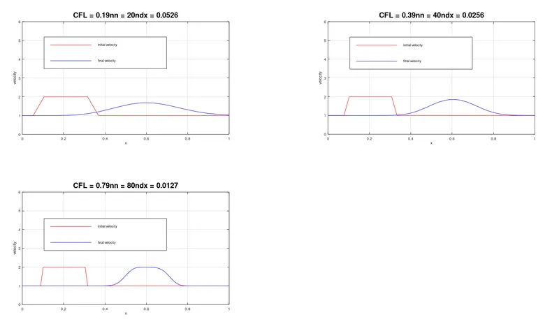
From the above graphs, we can conclude that as we increase the number of grid points 'n' the accuracy of the solution keeps increasing but after a certain value of 'n' the solution of the velocity profile will blowoff & the solution will become unstable.